
My Intro to Multiple Classification with Random Forests, Conditional Inference Trees, and Linear Discriminant Analysis
Want to share your content on R-bloggers? click here if you have a blog, or here if you don't.
After the work I did for my last post, I wanted to practice doing multiple classification. I first thought of using the famous iris dataset, but felt that was a little boring. Ideally, I wanted to look for a practice dataset where I could successfully classify data using both categorical and numeric predictors. Unfortunately it was tough for me to find such a dataset that was easy enough for me to understand.
The dataset I use in this post comes from a textbook called Analyzing Categorical Data by Jeffrey S Simonoff, and lends itself to basically the same kind of analysis done by blogger “Wingfeet” in his post predicting authorship of Wheel of Time books. In this case, the dataset contains counts of stop words (function words in English, such as “as”, “also, “even”, etc.) in chapters, or scenes, from books or plays written by Jane Austen, Jack London (I’m not sure if “London” in the dataset might actually refer to another author), John Milton, and William Shakespeare. Being a textbook example, you just know there’s something worth analyzing in it!! The following table describes the numerical breakdown of books and chapters from each author:
| # Books | # Chapters/Scenes | |
| Austen | 5 | 317 |
| London | 6 | 296 |
| Milton | 2 | 55 |
| Shakespeare | 12 | 173 |
Overall, the dataset contains 841 rows and 71 columns. 69 of those columns are the counted stop words (wow!), 1 is for what’s called the “BookID”, and the last is for the Author. I hope that the word counts are the number of times each word shows up per 100 words, or something that makes the counts comparable between authors/books.
The first thing I did after loading up the data into R was to create a training and testing set:
> authorship$randu = runif(841, 0,1)
> authorship.train = authorship[authorship$randu < .4,]
> authorship.test = authorship[authorship$randu >= .4,]
Then I set out to try to predict authorship in the testing data set using a Random Forests model, a Conditional Inference Tree model, and a Linear Discriminant Analysis model.
Random Forests Model
Here’s the code I used to train the Random Forests model (after finding out that the word “one” seemed to not be too important for the classification):
authorship.model.rf = randomForest(Author ~ a + all + also + an + any + are + as + at + be + been + but + by + can + do + down + even + every + for. + from + had + has + have + her + his + if. + in. + into + is + it + its + may + more + must + my + no + not + now + of + on + one + only + or + our + should + so + some + such + than + that + the + their + then + there + things + this + to + up + upon + was + were + what + when + which + who + will + with + would + your, data=authorship.train, ntree=5000, mtry=15, importance=TRUE)
It seemed to me that the mtry argument shouldn’t be too low, as we are trying to discriminate between authors! Following is a graph showing the Mean Decrease in Accuracy for each of the words in the Random Forests Model:
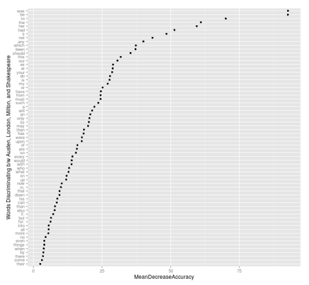
As you can see, some of the most important words for classification in this model were “was”, “be”, “to”, “the”, “her” and “had. At this point, I can’t help but think of the ever famous “to be, or not to be” line, and can’t help but wonder if these are the sort of words that would show up more often in Shakespeare texts. I don’t have the original texts to re-analyze, so I can only rely on what I have in this dataset to try to answer that question. Doing a simple average of how often the word “be” shows up per chapter per author, I see that it shows up an average of 12.9 times per scene in Shakespeare, and an average of 20.2 times per chapter in Austen! Shakespeare doesn’t win that game!!
Anyway, the Random Forests model does pretty well in classifying authors in the test set, as you can see in the counts and proportions tables below:
> authorship.test$pred.author.rf = predict(authorship.model.rf, authorship.test, type="response")
> table(authorship.test$Author, authorship.test$pred.author.rf)
> prop.table(table(authorship.test$Author, authorship.test$pred.author.rf),1)

              Austen London Milton Shakespeare
  Austen         182      4      0           0
  London           1    179      0           1
  Milton           0      1     33           2
  Shakespeare      1      2      0         102

                   Austen      London      Milton Shakespeare
  Austen      0.978494624 0.021505376 0.000000000 0.000000000
  London      0.005524862 0.988950276 0.000000000 0.005524862
  Milton      0.000000000 0.027777778 0.916666667 0.055555556
  Shakespeare 0.009523810 0.019047619 0.000000000 0.971428571
If you look on the diagonal, you can see that the model performs pretty well across authors. It seems to do the worst with Milton (although still pretty darned well), but I think that should be expected due to the low number of books and chapters from him.
Conditional Inference Tree
Here’s the code I used to train the Conditional Inference Tree model:
> authorship.model.ctree = ctree(Author ~ a + all + also + an + any + are + as + at + be + been + but + by + can + do + down + even + every + for. + from + had + has + have + her + his + if. + in. + into + is + it + its + may + more + must + my + no + not + now + of + on + one + only + or + our + should + so + some + such + than + that + the + their + then + there + things + this + to + up + upon + was + were + what + when + which + who + will + with + would + your, data=authorship.train)
Following is the plot that shows the significant splits done by the Conditional Inference Tree:

As is painfully obvious at first glance, there are so many end nodes that seeing the different end nodes in this graph is out of the question. Still useful however are the ovals indicating what words formed the significant splits. Similar to the Random Forests model, we see “be” and “was” showing up as the most significant words in discriminating between authors. Other words it splits on don’t seem to be as high up on the list in the Random Forests model, but the end goal is prediction, right?
Here is how the Conditional Inference Tree model did in predicting authorship in the test set:
> authorship.test$pred.author.ctree = predict(authorship.model.ctree, authorship.test, type="response")
> table(authorship.test$Author, authorship.test$pred.author.ctree)
> prop.table(table(authorship.test$Author, authorship.test$pred.author.ctree),1)

              Austen London Milton Shakespeare
  Austen         173      8      1           4
  London          18    148      3          12
  Milton           0      6     27           3
  Shakespeare      6     10      5          84

                   Austen      London      Milton Shakespeare
  Austen      0.930107527 0.043010753 0.005376344 0.021505376
  London      0.099447514 0.817679558 0.016574586 0.066298343
  Milton      0.000000000 0.166666667 0.750000000 0.083333333
  Shakespeare 0.057142857 0.095238095 0.047619048 0.800000000
Overall it looks like the Conditional Inference Tree model is doing a worse job predicting authorship compared with the Random Forests model (again, looking at the diagonal). Again we see the Milton records popping up as having the lowest hit rate for classification, but I think it’s interesting/sad that only 80% of Shakespeare records were correctly classified. Sorry old man, it looks like this model thinks you’re a little bit like Jack London, and somewhat like Jane Austen and John Milton.
Linear Discriminant Analysis
Finally we come to the real star of this particular show. Here’s the code I used to train the model:
> authorship.model.lda = lda(Author ~ a + all + also + an + any + are + as + at + be + been + but + by + can + do + down + even + every + for. + from + had + has + have + her + his + if. + in. + into + is + it + its + may + more + must + my + no + not + now + of + on + one + only + or + our + should + so + some + such + than + that + the + their + then + there + things + this + to + up + upon + was + were + what + when + which + who + will + with + would + your, data=authorship.train)
There’s a lot of summary information that the lda function spits out by default, so I won’t post it here, but I thought the matrix scatterplot of the records plotted along the 3 linear discriminants looked pretty great, so here it is:

From this plot you can see that putting all the words in the linear discriminant model seems to have led to pretty good discrimination between authors. However, it’s in the prediction that you see this model shine:
> authorship.test$pred.author.lda = predict(authorship.model.lda, authorship.test, type="response")
> authorship.test$pred.author.lda = predict(authorship.model.lda, authorship.test)$class
> table(authorship.test$Author, authorship.test$pred.author.lda)
> prop.table(table(authorship.test$Author, authorship.test$pred.author.lda),1)

              Austen London Milton Shakespeare
  Austen         185      1      0           0
  London           1    180      0           0
  Milton           0      0     36           0
  Shakespeare      0      0      0         105

                   Austen      London      Milton Shakespeare
  Austen      0.994623656 0.005376344 0.000000000 0.000000000
  London      0.005524862 0.994475138 0.000000000 0.000000000
  Milton      0.000000000 0.000000000 1.000000000 0.000000000
  Shakespeare 0.000000000 0.000000000 0.000000000 1.000000000
As you can see, it performed flawlessly with Milton and Shakespeare, and almost flawlessly with Austen and London.
Looking at an explanation of LDA from dtreg I’m thinking that LDA is performing best here because the discriminant functions created are more sensitive to the boundaries between authors (defined here by stop word counts) than the binary splits made on the predictor variables in the decision tree models. Does this hold for all cases of classification where the predictor variables are numeric, or does it break down if the normality of the predictors is grossly violated? Feel free to give me a more experienced/learned opinion in the comments!

R-bloggers.com offers daily e-mail updates about R news and tutorials about learning R and many other topics. Click here if you're looking to post or find an R/data-science job.
Want to share your content on R-bloggers? click here if you have a blog, or here if you don't.