[social4i size=”large” align=”float-right”]
Guest post by Christopher Johnson from www.codeitmagazine.com
One of the most powerful aspects of using R is that you can download free packages for so many tools and types of analysis. Text analysis is still somewhat in its infancy, but is very promising. It is estimated that as much as 80% of the world’s data is unstructured, while most types of analysis only work with structured data. In this paper, we will explore the potential of R packages to analyze unstructured text.
R provides two packages for working with unstructured text – TM and Sentiment. TM can be installed in the usual way. Unfortunately, Sentiment has been archived in 2012, and is therefore more difficult to install. However, it can still be installed using the following method, according to Frank Wang (Wang).
Once initially installed, each can be loaded later as library(name).
The next step is to load the data. I chose to download comments from a newspaper vent line (Charleston Gazette-Mail ). This data was saved to a text file and loaded and processed as follows.
###Get the data
data <- readLines("http://www.r-bloggers.com/wp-content/uploads/2016/01/vent.txt") # from: http://www.wvgazettemail.com/
df <- data.frame(data)
textdata <- df[df$data, ]
textdata = gsub("[[:punct:]]", "", textdata)
Next, we remove nonessential characters such as punctuation, numbers, web addresses, etc from the text, before we begin processing the actual words themselves. The code that follows was partially adapted from Gaston Sanchez in his work with sentiment analysis of Twitter data (Sanchez).
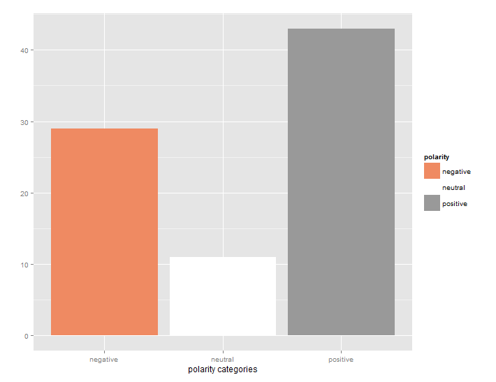
Next, we perform the sentiment analysis, classifying comments using a Bayesian analysis. A polarity of positive, negative, or neutral is determined. Finally, the comment, emotion, and polarity are combined in a single dataframe.
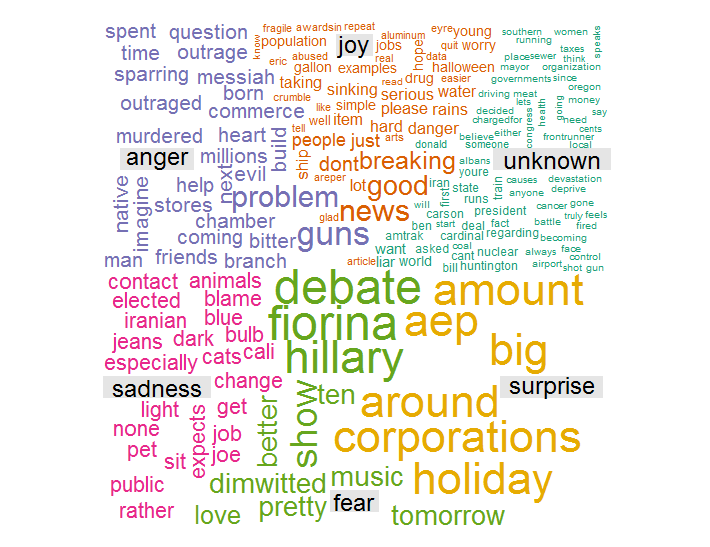
What do we gain from this analysis beside an attractive word cloud? We can analyze the word cloud itself. The Sentiment package has identified the most frequently occurring, important words, and their likely association with emotions. For instance, ‘guns’ was associated with anger, while ‘hillary’ was associated with fear. ‘pet’ was associate with sadness, and ‘aep’ was associated with surprise. With very little work, we have automatically extracted the important topics from the unstructured text.
More importantly, we also have a table of the comments themselves with the emotions and polarity attached. If we desire, we can sort them by emotion or polarity and continue our analysis. If this had been corporate satisfaction data, for example, we may want to dig deeper into angry comments and joyous comments for different reasons. We may use this as a tool to intelligently select comments for Quality Assurance analysis rather than blind random selection. Text and Sentiment Analysis may be in its infancy, but it is can also be the beginning for further analysis.


 We now prepare the data for creating a word cloud. This includes removing common English stop words.
 What do we gain from this analysis beside an attractive word cloud? We can analyze the word cloud itself. The Sentiment package has identified the most frequently occurring, important words, and their likely association with emotions. For instance, ‘guns’ was associated with anger, while ‘hillary’ was associated with fear. ‘pet’ was associate with sadness, and ‘aep’ was associated with surprise. With very little work, we have automatically extracted the important topics from the unstructured text.
More importantly, we also have a table of the comments themselves with the emotions and polarity attached. If we desire, we can sort them by emotion or polarity and continue our analysis. If this had been corporate satisfaction data, for example, we may want to dig deeper into angry comments and joyous comments for different reasons. We may use this as a tool to intelligently select comments for Quality Assurance analysis rather than blind random selection. Text and Sentiment Analysis may be in its infancy, but it is can also be the beginning for further analysis.
What do we gain from this analysis beside an attractive word cloud? We can analyze the word cloud itself. The Sentiment package has identified the most frequently occurring, important words, and their likely association with emotions. For instance, ‘guns’ was associated with anger, while ‘hillary’ was associated with fear. ‘pet’ was associate with sadness, and ‘aep’ was associated with surprise. With very little work, we have automatically extracted the important topics from the unstructured text.
More importantly, we also have a table of the comments themselves with the emotions and polarity attached. If we desire, we can sort them by emotion or polarity and continue our analysis. If this had been corporate satisfaction data, for example, we may want to dig deeper into angry comments and joyous comments for different reasons. We may use this as a tool to intelligently select comments for Quality Assurance analysis rather than blind random selection. Text and Sentiment Analysis may be in its infancy, but it is can also be the beginning for further analysis.