[social4i size=”large” align=”float-right”]
Guest post by Christopher Johnson from www.codeitmagazine.com
Some of my articles cover getting started with a particular software, and some cover tips and tricks for seasoned users. This article, however, is different. It does demonstrate the usage of an R package, but the main purpose is for fun.
In an article in Time, Matt Peckham described how French researchers were able to use four microphones and a single snap to model a complex room to within 1mm accuracy (Peckham). I decided that I wanted to attempt this (on a smaller scale) with one microphone and an R package. I was amazed at the results. Since the purpose of this article is not to teach anyone to write code to work with sound clips, rather than work with the code line by line, I will give a general overview, and I will present the code in full at the end for anyone that would like to recreate it for themselves.
The basic idea comes from the fact that sound travels at a constant speed in air. When it bounces off of an object, it returns in a predictable time. A microphone takes recordings at a consistent sampling rate, as well, which can be determined form the specs on the mic.
I placed a mic on my desk in a small office, pressed record, and snapped my fingers one time. I had an idea what to expect from my surroundings. The mic was placed on a desk, with a monitor about a foot away. There were two walls about three feet away and two walls and a ceiling about 6 feet away.
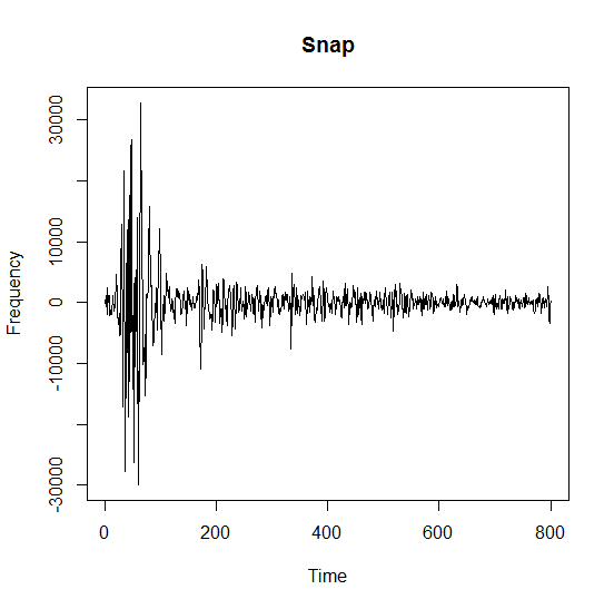
Next, I imported the sound clip into R. In R, there is a library called tuneR that enables us to work with sound clips. The following shows the initial image of the sound. Right away, we can see that there are several peaks that are larger than the others, which we would assume are the features we are interested in. The other peaks, we would assume, are smaller, less important, features of the room.
I wrote two functions to process the sound further. The first simply takes an observation, the sampling rate of the mic, and the speed of sound, and determines the distance traveled. The second function uses the first function to process a dataset of observations.
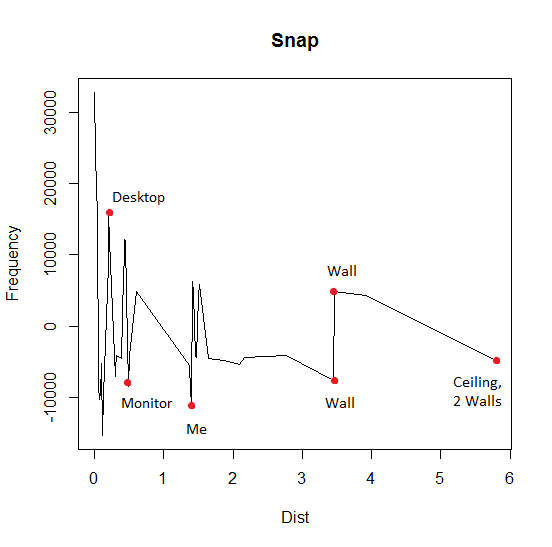
The output of this second function is a dataset of time and distances. Graphing this, we can more clearly see the results of our snap.
I have indicated the major features of the room, and they do indeed correspond to the expected distances from the room’s dimensions.
install.packages("tuneR", repos = "http://cran.r-project.org")
library(tuneR)
#Functions
sound_dist <- function(duration, samplingrate) {
  #Speed of sound is 1125 ft/sec
  return((duration/samplingrate)*1125/2)
}
sound_data <- function(dataset, threshold, samplingrate) {
  dataset <- snap@left
  threshold = 4000
  samplingrate = 44100
  data <- data.frame()
  max = 0
  maxindex = 0
  for (i in 1:length(dataset)) {
    if (dataset[i] > max) {
      max = dataset[i]
      maxindex = i
      data <- data.frame()
    }
    if (abs(dataset[i]) > threshold) {
      data <- rbind(data, c(i,dataset[i], sound_dist(i - maxindex, samplingrate)))
    }
  }
  colnames(data) <- c("x", "y", "dist")
  return(data)
}
#Analysis
snap <- readWave("Data/snap.wav")
print(snap)
play(snap)
plot(snap@left[30700:31500], type = "l", main = "Snap",
     xlab = "Time", ylab = "Frequency")
data <- sound_data(snap@left, 4000, 44100)
plot(data[,3], data[,2], type = "l", main = "Snap",
     xlab = "Dist", ylab = "Frequency")


 I wrote two functions to process the sound further. The first simply takes an observation, the sampling rate of the mic, and the speed of sound, and determines the distance traveled. The second function uses the first function to process a dataset of observations.
The output of this second function is a dataset of time and distances. Graphing this, we can more clearly see the results of our snap.
I wrote two functions to process the sound further. The first simply takes an observation, the sampling rate of the mic, and the speed of sound, and determines the distance traveled. The second function uses the first function to process a dataset of observations.
The output of this second function is a dataset of time and distances. Graphing this, we can more clearly see the results of our snap.
 I have indicated the major features of the room, and they do indeed correspond to the expected distances from the room’s dimensions.