
Inferring the community structure of networks
Want to share your content on R-bloggers? click here if you have a blog, or here if you don't.
I continue my little excursion into network science. In the last post, I gave a little introduction to simulating and visualizing undirected networks with community structure in R. In this post I want to explore a method to infer the community structure of a network from its adjacency matrix. That is, given that I know which nodes are connected to each other, I want to infer which nodes belong to the same community. I will focus on the case of two communities, but the method can be extended to three or more.
This post requires basic knowledge of matrix calculus, in particular eigen-decomposition. Understanding how the k-means clustering algorithm works is also useful. The R-code to reproduce all the figures is given at the bottom of the post.
The Laplacian of the adjacency matrix
Given N nodes of the network and their links, the adjacency matrix A is the N*N matrix whose element A_ij = 1 if node i is connected to node j, and A_ij = 0 otherwise. In an undirected network the adjacency matrix is symmetric, and since no “self-links” are allowed A_ii = 0 for all i.
In a network with community structure the adjacency matrix is block-diagonal, if the first n_1 nodes belong to community 1, the next n_2 links belong to community 2, and so on until n_K. Here is an example with K=2:
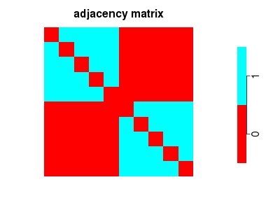
(If the labels of the nodes are not nicely ordered as above, the block-diagonal structure might not be immediately visible; I will come to this point later.)
The Laplacian L of the network is the N*N matrix that has L_ij = -1 if node i and j are connected and L_ij = 0 otherwise. The i-th diagonal element L_ii is equal to the total number of links of node i.
The Laplacian has a number of useful properties:
Look at the following block-diagonal Laplacian matrix with N=10, K=2 (5 nodes in each community) and its eigen-decomposition:
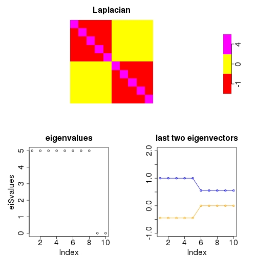
The eigenvalue spectrum shows that the last two eigenvalues are zero. The corresponding eigenvectors are shown as well (the blue one is shifted upwards by one unit). Their elements are constant inside the blocks.
In the following, we use the eigenvalue spectrum to infer the number of communities, and we use the eigenvectors to infer which nodes belong to which community.
Inferring the number of communities
As shown above, the number of blocks of the Laplacian can be inferred from the number of vanishing eigenvalues if the block-diagonal structure is perfect. If there are links between nodes in different communities, the Laplacian is only approximately block-diagonal since some off-diagonal elements are nonzero. Therefore, last few eigenvalues will not vanish exactly, but they will be close to zero. The following Laplacian corresponds to a the same network as above, but where the link between nodes 1 and 2 has been deleted, and a link between nodes 3 and 9 has been added.
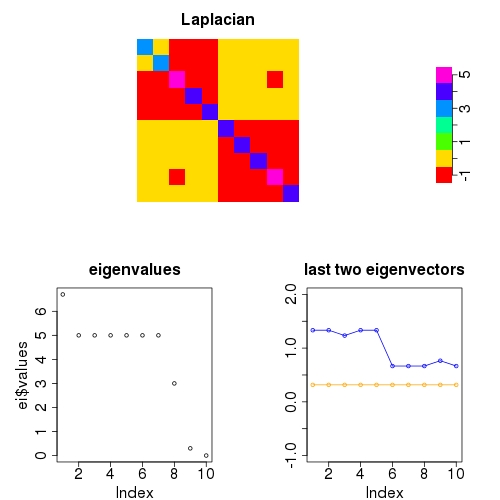
The number of small eigenvalues, and thus the number of communties can be chosen by “eyeballing” the eigenvalue spectrum for where the cutoff occurs. Or one can automate the selection of K.
I found that the k-means clustering algorithm (R implementation stats::kmeans) can be used to determine the cutoff. The idea is that the eigenvalue spectrum is quite smooth until a sharp cutoff appears before the almost-vanishing eigenvalues. This cutoff divides the eigenvalues into two clusters and we can make the k-means algorithm look for exactly two clusters. For the above eigenvalue spectrum, k-means correctly finds the size of the smaller cluster to be 2:
>> ei <- eigen(laplacian)
>> kmeans(ei$values,centers=range(ei$values))
...
 Clustering vector:
 [1]  2 2 2 2 2 2 2 2 1 1
...
Inferring the community structure
I shuffled the labels of the nodes in the figure above but kept their links unchanged. The new Laplacian and its eigen-decomposition now looks as follows:

Do you still see the community structure in the Laplacian? I don’t. But one of the eigenvectors can see it.
There are still two very small eigenvalues, indicating two communities, which is the correct number.
The second to last eigenvector (blue) indicates the community structure. Running the k-means clustering algorithm on the elements of this vector yields:
>> kmeans(ei$vectors[,9],centers=range(ei$vectors[,9]))
...
 Clustering vector:
 [1]   1 1 2 1 2 1 2 2 2 1
...
For comparison, the original node labels were
>> shuf.ind
 [1]  6  7  1 10  4  8  3  2  5  9
That is nodes 1,2,4,6 and 10 (which correspond to nodes 6-10 under the original labeling) are put into one cluster and the others respectively. By applying the k-means algorithm to the eigenvector elements, we reconstructed the community structure perfectly. I found this method to work also for larger values of N. If K increases, you will have to apply the above procedure iteratively. If more links exist between nodes in different communities, misclassification or overestimation of the number of communities occurs.
The goal of this post was to illustrate a naive method for inferring unknown network properties, namely the community structure. All I know about the network Laplacian and its eigen-decomposition is based on reference [1]. No thourough testing of the above method was performed, and I have no detailed results about misclassification behavior or under/over-estimation of the number of clusters. Please check [1] and references therein if you are curious about more advanced methods for community detection.
I find the above method quite visual and understandable. In case the k-means algorithm returns completely unreasonable results, the number of nodes and the separation of the eigenvector elements could as well be performed by hand if the number of communities is small. I consider this a useful property which more advance methods might not have.
If you find errors or something that remained unclear, feel free to leave a comment. This is it, thanks for watching.
References
[1] Newman (2004) Detecting community structure in networks, Eur. Phys. J. B 38, DOI:10.1140/epjb/e2004-00124-y
The R code to produce the above figures:
graphics.off()
JPG <- TRUE

#################################
# block-diagonal adjacency matrix
# Figure 1
#################################

if (JPG) {
    jpeg("adjacency-mat.jpg",width=400,height=300,quality=100)
} else {
    x11()
}
par(cex.lab=2,cex.main=2,cex.axis=2)
#construct block diagonal adjacency matrix
v1 <- c(rep(1,5),rep(0,5))
v2 <- c(rep(0,5),rep(1,5))
blomat <- rbind(v1,v1,v1,v1,v1,v2,v2,v2,v2,v2)
diag(blomat) <- 0
layout(t(c(1,1,1,1,2)))
#plot adj. matrix
image(blomat[,10:1],asp=1,axes=F,col=rainbow(2), main="adjacency matrix")
#colorbar
par(mar=c(7,2,7,5))
image(matrix(seq(2),ncol=2),axes=F,col=rainbow(2))
axis(side=4,at=seq(0,1,length.out=2),labels=paste(c(0,1)), cex.axis=2)
if (JPG) dev.off()


############################
# perfect two block laplacian + eigenspectrum
# Figure 2
############################
#construct laplacian
laymat <- rbind(c(1,1,1,1,1,2),c(3,3,3,4,4,4))
v1 <- c(rep(-1,5),rep(0,5))
v2 <- c(rep(0,5),rep(-1,5))
blomat <- rbind(v1,v1,v1,v1,v1,v2,v2,v2,v2,v2)
diag(blomat) <- 4
if (JPG) {
    jpeg("laplace-perfect.jpg",width=500,height=500, quality=100)
} else {
    x11()
}
par(cex.lab=2,cex.main=2,cex.axis=2)
layout(laymat)
#plot laplacian
image(blomat[,10:1],asp=1,axes=F,col=rainbow(6), main="Laplacian")
#colorbar
par(mar=c(7,2,7,5))
image(matrix(seq(3),ncol=3),axes=F,col=rainbow(6)[c language="(1,2,6)"][/c])
axis(side=4,at=seq(0,1,length.out=3),labels=paste(c(-1,0,4)), cex.axis=2)
par(mar=c(4,6,4,4))
#eigendecomp.
ei <- eigen(blomat)
#plot eigenvalues
plot(ei$values,main="eigenvalues")
#plot eigenvectors
plot(NULL,xlim=c(1,10),ylim=c(-1,2),main="last two eigenvectors", ylab=NA)
lines(ei$vectors[,9]+1,type="o",col="blue")
lines(ei$vectors[,10],type="o",col="orange")
if (JPG) dev.off()

############################
# block-diagonal laplacian with impurities
# Figure 3
############################
#construct the laplacian
v1 <- c(rep(-1,5),rep(0,5))
v2 <- c(rep(0,5),rep(-1,5))
blomat <- rbind(v1,v1,v1,v1,v1,v2,v2,v2,v2,v2)
blomat[1,2] <- blomat[2,1]<- 0
blomat[3,9] <- blomat[9,3]<- -1
diag(blomat) <- 0
diag(blomat) <- -colSums(blomat)
if (JPG) {
    jpeg("laplace-imperfect.jpg",width=500,height=500, quality=100)
} else {
    x11()
}
par(cex.lab=2,cex.main=2,cex.axis=2)
layout(laymat)
#plot the laplacian
image(blomat[,10:1],asp=1,axes=F,col=rainbow(7), main="Laplacian")
par(mar=c(7,2,7,5))
#colorbar
image(matrix(seq(7),ncol=7),axes=F,col=rainbow(7))
axis(side=4,at=seq(0,1,length.out=7),labels=paste(seq(-1,5)), cex.axis=2)
par(mar=c(4,6,4,4))
#eigendecomposition and k-means clustering
ei <- eigen(blomat)
print(kmeans(ei$values,range(ei$values)))
#plot eigenvalues
plot(ei$values,main="eigenvalues")
#plot eigenvectors
plot(NULL,xlim=c(1,10),ylim=c(-1,2), main="last two eigenvectors", ylab=NA)
lines(ei$vectors[,9]+1,type="o",col="blue")
lines(ei$vectors[,10],type="o",col="orange")
if (JPG) dev.off()


###############################
#disordered block-diagonal laplacian with impurities
# Figure 4
###############################
#construct Laplacian
v1 <- c(rep(-1,5),rep(0,5))
v2 <- c(rep(0,5),rep(-1,5))
blomat <- rbind(v1,v1,v1,v1,v1,v2,v2,v2,v2,v2)
blomat[1,2] <- blomat[2,1]<- 0
blomat[3,9] <- blomat[9,3]<- -1
shuf.ind <- c(6, 7, 1, 10, 4, 8, 3, 2, 5, 9)
blomat <- blomat[shuf.ind, shuf.ind]
diag(blomat) <- 0
diag(blomat) <- -rowSums(blomat)

if (JPG) {
    jpeg("laplace-disordered.jpg",width=500,height=500, quality=100)
} else {
    x11()
}
par(cex.lab=2,cex.main=2,cex.axis=2)
layout(laymat)
#plot Laplacian
image(blomat[,10:1],asp=1,axes=F,col=rainbow(7), main="Laplacian")
par(mar=c(7,2,7,5))
#plot colorbar
image(matrix(seq(7),ncol=7),axes=F,col=rainbow(7))
axis(side=4,at=seq(0,1,length.out=7),labels=paste(seq(-1,5)), cex.axis=2)
par(mar=c(4,6,4,4))
#eigendecomposition
ei <- eigen(blomat)
#plot eigenvalues
plot(ei$values,main="eigenvalues")
#plot eigenvectors
plot(NULL,xlim=c(1,10),ylim=c(-1,2), main="last two eigenvectors", ylab=NA)
lines(ei$vectors[,9]+1,type="o",col="blue")
lines(ei$vectors[,10],type="o",col="orange")
if (JPG) dev.off()
R-bloggers.com offers daily e-mail updates about R news and tutorials about learning R and many other topics. Click here if you're looking to post or find an R/data-science job.
Want to share your content on R-bloggers? click here if you have a blog, or here if you don't.