```{r Data_prep, echo=FALSE, message=FALSE, warning=FALSE}
# Moved this outside the document for easy of reading
# I often have those sections in here
source("Setup_and_munge.R")
```
 
```{r Versions}
info <- sessionInfo()
r_ver <- paste(info$R.version$major, info$R.version$minor, sep=".")
```
 
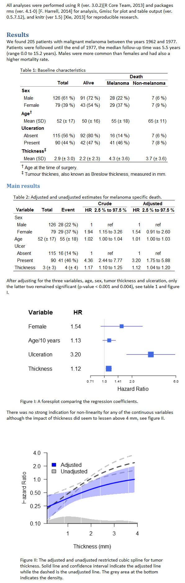
All analyses were performed using R (ver. `r r_ver`)[R Core Team, 2013] 
and packages rms (ver. `r info$otherPkgs$rms$Version`) [F. Harrell, 2014] 
for analysis, Gmisc for plot and table output (ver. `r info$otherPkgs$Gmisc$Version`), 
and knitr (ver `r info$otherPkgs$knitr$Version`) [Xie, 2013] for reproducible research.
 
Results
=======
 
We found `r nrow(melanoma)` patients with malignant melanoma between the years 
`r paste(range(melanoma$year), collapse=" and ")`. Patients were followed until 
the end of 1977, the median follow-up time was `r sprintf("%.1f", median(melanoma$time_years))` 
years (range `r paste(sprintf("%.1f", range(melanoma$time_years)), collapse=" to ")` years). 
Males were more common than females and had also a higher mortality rate.
 
```{r Table1, results='asis', cache=FALSE}
table_data <- list()
getT1Stat <- function(varname, digits=0){
  getDescriptionStatsBy(melanoma[, varname], melanoma$status, 
                        add_total_col=TRUE,
                        show_all_values=TRUE, 
                        hrzl_prop=TRUE,
                        statistics=FALSE, 
                        html=TRUE, 
                        digits=digits)
}
 
# Get the basic stats
table_data[["Sex"]] <- getT1Stat("sex")
table_data[["Age<sup>†</sup>"]] <- getT1Stat("age")
table_data[["Ulceration"]] <- getT1Stat("ulcer")
table_data[["Thickness<sup>‡</sup>"]] <- getT1Stat("thickness", digits=1)
 
# Now merge everything into a matrix
# and create the rgroup & n.rgroup variabels
rgroup <- c()
n.rgroup <- c()
output_data <- NULL
for (varlabel in names(table_data)){
  output_data <- rbind(output_data, table_data[[varlabel]])
  rgroup <- c(rgroup, varlabel)
  n.rgroup <- c(n.rgroup, nrow(table_data[[varlabel]]))
}
 
# Add a column spanner for the death columns
cgroup <- c("", "Death")
n.cgroup <- c(2, 2)
colnames(output_data) <- gsub("[ ]*death", "", colnames(output_data))
 
htmlTable(output_data, align="rrrr",
          rgroup=rgroup, n.rgroup=n.rgroup, 
          rgroupCSSseparator="", 
          cgroup = cgroup,
          n.cgroup = n.cgroup,
          rowlabel="", 
          caption="Baseline characteristics", 
          tfoot=paste0("<sup>†</sup> Age at the time of surgery.",
                       " <br/><sup>‡</sup> Tumour thicknes,",
                       " also known as Breslow thickness, measured in mm."), 
          ctable=TRUE)
```
 
Main results
------------
 
```{r C_and_A, results='asis'}
# Setup needed for the rms coxph wrapper
ddist <- datadist(melanoma)
options(datadist = "ddist")
 
# Do the cox regression model 
# for melanoma specific death
msurv <- Surv(melanoma$time_years, melanoma$status=="Melanoma death")
fit <- cph(msurv ~ sex + age + ulcer + thickness, data=melanoma)
 
# Print the model
printCrudeAndAdjustedModel(fit, desc_digits=0,
                           caption="Adjusted and unadjusted estimates for melanoma specific death.",
                           desc_column=TRUE,
                           add_references=TRUE, 
                           ctable=TRUE)
 
pvalues <- 
  1 - pchisq(coef(fit)^2/diag(vcov(fit)), df=1)
```
 
```{r}
pvalue_formatter <- function(pvalues, sig.limit = 0.001){
  sapply(pvalues, function(x, sig.limit){
    if (x < sig.limit)
      return(sprintf("< %s", format(sig.limit))) 
    # < stands for < and is needed
    # for the markdown/html to work
    # and the format is needed to avoid trailing zeros
 
    # High p-values you usually want two decimals
    # otherwise report only one
    if (x > 0.01)
      return(format(x, digits=2))
 
    return(format(x, digits=1))
    }, sig.limit=sig.limit)
}
```
 
After adjusting for the three variables, age, sex, tumor thickness 
and ulceration, only the latter two remained significant (p-value 
`r pvalue_formatter(pvalues["ulcer=Present"])` and 
`r pvalue_formatter(pvalues["thickness"])`), 
see table `r as.numeric(options("table_counter"))-1` 
and figure `r getNextFigureNo()`.
 
```{r Regression_forestplot, fig.height=3, fig.width=5, fig.cap="A foresplot comparing the regression coefficients."}
# I've adjusted the coefficient for age to be by 
forestplotRegrObj(update(fit, .~.-age+I(age/10)), 
                  order.regexps=c("Female", "age", "ulc", "thi"),
                  box.default.size=.25, xlog=TRUE,
                  new_page=TRUE, clip=c(.5, 6), rowname.fn=function(x){
  if (grepl("Female", x))
    return("Female")
 
  if (grepl("Present", x))
    return("Ulceration")
 
  if (grepl("age", x))
    return("Age/10 years")
 
  return(capitalize(x))
})
```
 
There was no strong indication for non-linearity for any of the 
continuous variables although the impact of thickness did 
seem to lessen above 4 mm, see figure `r getNextFigureNo()`.
 
```{r spline_plot, fig.cap=plotHR_cap}
plotHR_cap = paste0("The adjusted and unadjusted restricted cubic spline",
                    " for tumor thickness. Solid line and confidence interval",
                    " indicate the adjusted line while the dashed is",
                    " the unadjusted line. The grey area at ",
                    " the bottom indicates the density.")
# Generate adjusted and anuadjusted regression models
rcs_fit <- update(fit, .~.-thickness+rcs(thickness, 3))
rcs_fit_ua <- update(fit, .~+rcs(thickness, 3))
 
# Make sure the axes stay at the exact intended points
par(xaxs="i", yaxs="i")
plotHR(list(rcs_fit, rcs_fit_ua), col.dens="#00000033",
       lty.term=c(1, 2),
       col.term=c("blue", "#444444"), 
       col.se = c("#0000FF44", "grey"),
       polygon_ci=c(TRUE, FALSE),
       term="thickness", 
       xlab="Thickness (mm)", 
       ylim=c(.1, 4), xlim=c(min(melanoma$thickness), 4), 
       plot.bty="l", y.ticks=c(.1, .25, .5, 1, 2, 4))
legend(x=.1, y=1.1, legend=c("Adjusted", "Unadjusted"), fill=c("blue", "grey"), bty="n")
```

##################
# Knitr settings #
##################
 
# Load the knitr package so that the code
# doesn't complain outside knitr
library(knitr) 
 
# Set some basic options. You usually do not
# want your code, messages, warnings etc
# to show in your actual manuscript
opts_chunk$set(warning=FALSE, 
               message=FALSE, 
               echo=FALSE, 
               dpi=96,
               fig.width=4, fig.height=4, # Default figure widths
               dev="png", dev.args=list(type="cairo"), # The png device
               # Change to dev="postscript" if you want the EPS-files
               # for submitting. Also remove the dev.args() as the postscript
               # doesn't accept the type="cairo" argument.
               error=FALSE)
 
# Evaluate the figure caption after the plot
opts_knit$set(eval.after='fig.cap')
 
# Avoid including base64_images - this only 
# works with the .RProfile setup
options(base64_images = "none")
 
# Use the table counter that the htmlTable() provides
options(table_counter = TRUE)
 
# Use the figure counter that we declare below
options(figure_counter = TRUE)
# Use roman letters (I, II, III, etc) for figures
options(figure_counter_roman = TRUE)
 
# Adding the figure number is a little tricky when the format is roman
getNextFigureNo <- function() as.character(as.roman(as.numeric(options("figure_counter"))))
 
# Add a figure counter function
knit_hooks$set(plot = function(x, options) {
  fig_fn = paste0(opts_knit$get("base.url"), 
                  paste(x, collapse = "."))
 
  # Some stuff from the default definition
  fig.cap <- knitr:::.img.cap(options)
 
  # Style and additional options that should be included in the img tag
  style=c("display: block",
          sprintf("margin: %s;",
                   switch(options$fig.align, 
                          left = 'auto auto auto 0', 
                          center = 'auto',
                          right = 'auto 0 auto auto')))
  # Certain arguments may not belong in style, 
  # for instance the width and height are usually
  # outside if the do not have a unit specified
  addon_args = ""
 
  # This is perhaps a little overly complicated prepared 
  # with the loop but it allows for a more out.parameters if necessary
  if (any(grepl("^out.(height|width)", names(options)))){
      on <- names(options)[grep("^out.(height|width)", names(options))]
      for(out_name in on){
          dimName <- substr(out_name, 5, nchar(out_name))
          if (grepl("[0-9]+(em|px|%|pt|pc|in|cm|mm)", out_name))
              style=append(style, paste0(dimName, ": ", options[[out_name]]))
          else if (length(options$out.width) > 0)
              addon_args = paste0(addon_args, dimName, "='", options[[out_name]], "'")
      }
  }
 
  # Add counter if wanted
  fig_number_txt <- ""
  cntr <- getOption("figure_counter", FALSE)
  if (cntr != FALSE){
    if (is.logical(cntr))
      cntr <- 1
    # The figure_counter_str allows for custom 
    # figure text, you may for instance want it in
    # bold: <b>Figure %s:</b>
    # The %s is so that you have the option of setting the
    # counter manually to 1a, 1b, etc if needed
    fig_number_txt <- 
      sprintf(getOption("figure_counter_str", "Figure %s: "), 
              ifelse(getOption("figure_counter_roman", FALSE), 
                     as.character(as.roman(cntr)), as.character(cntr)))
 
    if (is.numeric(cntr))
      options(figure_counter = cntr + 1)
  }
 
  # Put it all together
  paste0("<figure><img src='", fig_fn, "'", 
         " ", addon_args,
         paste0(" style='", paste(style, collapse="; "), "'"),
         ">",
         "<figcaption>", fig_number_txt, fig.cap, "</figcaption></figure>")
})
 
#################
# Load_packages #
#################
library(rms) # I use the cox regression from this package
library(boot) # The melanoma data set is used in this exampe
library(Gmisc) # Stuff I find convenient
 
##################
# Munge the data #
##################
 
# Here we go through and setup the variables so that
# they are in the proper format for the actual output
 
# Load the dataset - usually you would use read.csv
# or something similar
data("melanoma")
 
# Set time to years instead of days
melanoma$time_years <- 
  melanoma$time / 365.25
 
# Factor the basic variables that 
# we're interested in
melanoma$status <- 
  factor(melanoma$status, 
         levels=c(2, 1, 3),
         labels=c("Alive", # Reference
                  "Melanoma death", 
                  "Non-melanoma death"))
melanoma$sex <- 
  factor(melanoma$sex,
         labels=c("Male", # Reference
                  "Female"))
 
melanoma$ulcer <- 
  factor(melanoma$ulcer,
         levels=0:1,
         labels=c("Absent", # Reference
                  "Present"))