Anytime I get a new hammer, I waste no time in trying to find something to bash with it. Prior to last year, I wouldn’t have known what a cluster was, other than the first half of a slang term used to describe a poor decision-making process. Now I’ve seen it in action a few times and have searched for a practical case where I could use it. It occurred to me that it made for a very interesting look at the problem of how to group loss development factors.

As I may have ranted previously, I’ve tried to revert to first principles and challenge the notion that every development lag deserves its own model factor. Moreover, I’m not 100% satisfied with the idea that development age is the ideal way to categorize model factors. Just for fun, let’s see how a k-means clustering algorithm would group loss development factors.

We’ll work with data from a “big company” pulled from the public NAIC data set. (The data set and the logic to create the Triangle object are available in the MRMR package, which is on GitHub here.)

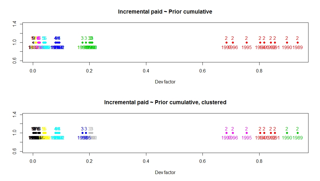
First, we’ll calculate the development factors using a standard multiplicative chain ladder model. For a 10×10 loss triangle, we’ll have 45 factors. We can plot them on the real number line to see where they sit relative to one another. We’re going to display two plots. The upper plot will show the factors colored by development lag. The numbers are listed above as a further guide to the identity of the points. Development lags 2, 3 and 4 appear clustered in groups, but the higher lags are a bit more difficult to distinguish.

The lower plot shows the dots colored based on their assignment to clusters using the kmeans function. The 2nd and 3rd lags are now divided into finer clusters. Also, the 7 through 10 factors in the tail now sort together. (This is a bit difficult to see. Suggestions on how to present this more clearly are welcome.)

Development lag 2 is particularly interesting as it’s the largest factor and the one with the greatest volatility. I’m curious if the clustering suggests something happening as a calendar year effect, or if it’s merely an artifact of the kmeans clustering algorithm (garbage in, garbage out, etc.). So, let’s add a label for the calendar periods. When we do this, we see that lag 2 does appear to have a meaningful calendar period effect. 1989 and 1990 sort together, then there is a cluster from 1991-1994 and a final cluster for calendar years 1995-1997.

The higher lags are more difficult to see, but let’s have a look at lag 3 and higher. Again we notice that calendar years 1995-1997 get sorted apart from the others. At this point, we should have a strong suspicion that there is a calendar year trend which affects our loss development pattern, though the effect may be dampened for higher lags. We can account for this in a number of ways- Berquist-Sherman adjustment or use of a Zehnwirth type fitting formula.

Note that we’ll get different results whenever we run the kmeans algorithm. Your mileage may vary.

The code is long and not all that interesting, however I welcome any comments. You can find the Gist here.