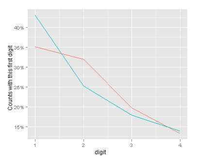
Benford’s Law after converting count data to be in base 5

Firstly, I know nothing about election fraud – this isn’t a serious post. But, I do like to do some simple coding. Ben Goldacre posted on using Benford’s Law to look for evidence of Russian election fraud. Then Richie Cotton did the same, but using R. Commenters on both sites suggested that as the data didn’t span a large order of magnitude, turning it into a lower base (e.g. base 5) may helpful. I’ve no idea if this would be helpful, but the idea of messing around with the data was appealing, so here it is.

The as.binary() function was posted to R-help by Robin Hankin. The code to do the analysis was by Richie Cotton. Putting it all together gives:

So there we have it – with the numerical data in base 5, the observed and expected values are closer together than with the numerical data in base 10. The overall dynamic range is from 1 to 30430 (in base 5).

The data are here. The code you’ll need is:-

 
## repeat the analysis but with base 5
rm(list = ls())
library(reshape)
library(stringr)
library(ggplot2)
russian <- read.csv("Russian observed results - FullData.csv")

as.binary <- function(n,base=2 , r=FALSE){ 
  ## function written by robin hankin
  out <- NULL 
  while(n > 0) { 
    if(r) { 
      out <- c(out , n%%base) 
    } else { 
      out <- c(n%%base , out) 
    } 
    n <- n %/% base 
  } 
  ans <- str_c(out, collapse = "")
  return(ans)
}
russian <- melt(
  russian[, 9:13], 
  variable_name = "candidate"
  )
russian$base_5_value <- apply(as.matrix(russian$value), MARGIN = 1,
                              FUN = as.binary, base = 5)
russian$base_5_value_1st = str_extract(russian$base_5_value, "[123456789]")

first_digit_counts <- as.vector(table(russian$base_5_value_1st))

first_digit_actual_vs_expected <- data.frame(
  digit            = 1:4,
  actual.count     = first_digit_counts,   
  actual.fraction  = first_digit_counts / nrow(russian),
  benford.fraction = log(1 + 1 / (1:4), base = 5)
  )

a_vs_e <- melt(first_digit_actual_vs_expected[, c("digit", "actual.fraction", "benford.fraction")], id.var = "digit")
(fig1_lines <- ggplot(a_vs_e, aes(digit, value, colour = variable)) +
  geom_line() +
  scale_x_continuous(breaks = 1:4) +
  scale_y_continuous(formatter = "percent") +
  ylab("Counts with this first digit") +
  opts(legend.position = "none")
 )

range(as.numeric(russian$base_5_value), na.rm = T)