Following Arthur Charpentier‘s example, I am going to try to post occasionally on material covered during my courses, in the hope that it might be useful to my students, but also to others.

In the second practical of the Bayesian Case Studies course, we looked at Bayesian model choice and basic Monte Carlo methods, looking at data about the number of oral questions asked by French deputies (Members of Parliament). We wanted to know whether male and female deputies behave differently in this matter. If we model the number of questions asked by a deputy by a Poisson random variable and denote their gender (1 for men, 2 for women), we thus need to choose between the following two models. (See the course website for the question sheet and other material; the slides are below.)

Model 1:

Model 2:

First download the data and set some variables:

 > deputes=read.csv2('http://www.ceremade.dauphine.fr/~ryder/CaseStudies/deputes.csv')
 > attach(deputes)#Q1
 > summary(questions_orales)
 > hist(questions_orales,breaks=(0:6-.5))
 > (n=length(questions_orales))
 > (nh=sum(sexe=="H"))
 > (nf=sum(sexe=="F"))
 > (qtot=sum(questions_orales))
 > (qh=sum(questions_orales[sexe=="H"]))
 > (qf=sum(questions_orales[sexe=="F"]))

Since the Gamma prior is a conjugate prior for the Poisson model, we get a Gamma distribution as our posterior. Using a as prior, here is a comparison of the prior and the posteriors for the two models (in the bottom plot, is in black and in red.

Two observations here: First, the posterior is much more peaked than the prior, which is expected since the number of data points is large. Second, in model 2, it seems that there may be a difference between men and women, with women asking slightly less questions in Parliament.To verify this, we compute a Bayes factor to compare the two models. In this case, the Bayes factor is available in closed form, but an initial computation does not work because is too large:

> BF_analytical=function(a,b,y1,n1,y2,n2){
+   m1=b^a/gamma(a)*gamma(a+y1+y2)/(b+n1+n2)^(a+y1+y2)
+   m2=b^(2*a)/gamma(a)^2*gamma(a+y1)/(b+n1)^(a+y1)*gamma(a+y2)/(b+n2)^(a+y2)
+   return(m2/m1)
+ }
> BF_analytical(2,2,qh,nh,qf,nf)
[1] NaN
Warning messages:
1: In BF_analytical(2, 2, qh, nh, qf, nf) :
  value out of range in 'gammafn'
2: In BF_analytical(2, 2, qh, nh, qf, nf) :
  value out of range in 'gammafn'

However, we are able to compute the Bayes factor analytically by using the log-scale instead.

> BF_analytical2=function(a,b,y1,n1,y2,n2){
+   m1=a*log(b)-lgamma(a)+lgamma(a+y1+y2)-(a+y1+y2)*log(b+n1+n2)
+   m2=2*a*log(b)-2*lgamma(a)+lgamma(a+y1)-(a+y1)*log(b+n1)+lgamma(a+y2)-(a+y2)*log(b+n2)
+   return(exp(m2-m1))
+ }
> BF_analytical2(2,2,qh,nh,qf,nf)
[1] 0.1875569
> log10(BF_analytical2(2,2,qh,nh,qf,nf))
[1] -0.726867

Using Jeffrey’s scale of evidence, this corresponds to “substantial” evidence in favour of model 1 (i.e. no difference between men and women).

Even if we had not been able to calculate the Bayes factor exactly, we could have approximated it using Monte Carlo. We first create two functions to calculate the likelihood under model 1 and model 2, and start with vanilla Monte Carlo.

> lkd.model1=function(y,n,lambda){  return(exp(-n*lambda+y*log(lambda))) }
> lkd.model2=function(y1,n1,y2,n2,lambda1,lambda2){  return(exp(-n1*lambda1+y1*log(lambda1)-n2*lambda2+y2*log(lambda2))) }

> BF_MC=function(a,b,y1,n1,y2,n2,M){
 +  lambda1=rgamma(M,a,b)
 +  m1=cumsum(lkd.model1(y1+y2,n1+n2,lambda1))/(1:M)
 + lambda2.1=rgamma(M,a,b)
 + lambda2.2=rgamma(M,a,b)
 +  m2=cumsum(lkd.model2(y1,n1,y2,n2,lambda2.1,lambda2.2))/(1:M)
 +  return(m2/m1)
 + }

> M=100000
> BF_MC(2,2,qh,nh,qf,nf,M)[M]
[1] 0.1776931
> plot(100:M,BF_MC(2,2,qh,nh,qf,nf,M)[100:M], type="l")

The last line creates a plot of how our Monte Carlo estimate of the Bayes factor changes as the number of iterations increases. It is useful to check convergence.

Here, it is clear that the method converges after a few tens of thousands iterations. Our estimate for is close to the true value (two decimal places precision). Next, we try the harmonic mean method:

> BF_HM=function(a,b,y1,n1,y2,n2,M){
+   lambda1=rgamma(M,a+y1+y2,b+n1+n2)
+   m1=(1:M)/(cumsum(1/lkd.model1(y1+y2,n1+n2,lambda1)))
 +  lambda2.1=rgamma(M,a+y1,b+n1)
 +  lambda2.2=rgamma(M,a+y2,b+n2)
 +  m2=(1:M)/cumsum(1/lkd.model2(y1,n1,y2,n2,lambda2.1,lambda2.2))
+   return(m2/m1)  
+ }

> BF_HM(2,2,qh,nh,qf,nf,M)[M]
[1] 0.2451013
> plot(100:M,BF_HM(2,2,qh,nh,qf,nf,M)[100:M], type="l")

We observe that this does not appear to converge. It is known that in general, the harmonic mean method is unreliable.

We finally move on to importance sampling. In importance sampling, we want to estimate where by using simulations from an alternate density . This will be most efficient when is close to $h\times f$. In this case, we therefore need to be similar to the posterior distribution, so we take a normal density with mean and variance the same as the posterior distribution:

> BF_IS=function(a,b,y1,n1,y2,n2,M){
+  mean1=(a+y1+y2)/(b+n1+n2)
+  mean2.1=(a+y1)/(b+n1)
+  mean2.2=(a+y2)/(b+n2)

+  sigma1=sqrt((a+y1+y2)/(b+n1+n2)^2)
+  sigma2.1=sqrt((a+y1)/(b+n1)^2)
+  sigma2.2=sqrt((a+y2)/(b+n2)^2)

+  lambda1=rnorm(M,mean1,sigma1)
+  m1=cumsum( lkd.model1(y1+y2,n1+n2,lambda1) * dgamma(lambda1,a, b) / dnorm(lambda1,mean1,sigma1))/(1:M)

+  lambda2.1=rnorm(M,mean2.1, sigma2.1)
+  lambda2.2=rnorm(M,mean2.2, sigma2.2)
+  m2=cumsum( lkd.model2(y1,n1,y2,n2,lambda2.1,lambda2.2) * dgamma(lambda2.1,a, b) * dgamma(lambda2.2,a,b) / 
+    (dnorm(lambda2.1,mean2.1,sigma2.1)*dnorm(lambda2.2,mean2.2,sigma2.2))) / (1:M)

+  return(m2/m1)
+ }

> BF_IS(2,2,qh,nh,qf,nf,M)[M]
[1] 0.1875875
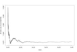
> plot(100:M,BF_IS(2,2,qh,nh,qf,nf,M)[100:M], type="l")

This method converges. Note that the y-scale is much tighter than for vanilla Monte Carlo: convergence is in fact much faster, and we get a more precise estimate than by using vanilla Monte Carlo. This is more obvious if we look at both methods on the same graph.

> plot(100:M,BF_MC(2,2,qh,nh,qf,nf,M)[100:M], type="l") 
> lines(100:M,BF_IS(2,2,qh,nh,qf,nf,M)[100:M], col="red")

It is much more visible now that importance sampling is a clear winner.

With this computation of the Bayes factor, we choose model 1: a single parameter can be used to model the behaviour of men and women.