
A Visualization of World Cuisines
Want to share your content on R-bloggers? click here if you have a blog, or here if you don't.
In a previous post, we had ‘mapped’ the culinary diversity in India through a visualization of food consumption patterns. Since then, one of the topics in my to-do list was a visualization of world cuisines. The primary question was similar to that asked of the Indian cuisine: Are cuisines of geographically and culturally closer regions also similar? I recently came across an article on the analysis of recipe ingredients that distinguish the cuisines of the world. The analysis was conducted on a publicly available dataset consisting of ingredients for more than 13,000 recipes from the recipe website Epicurious. Each recipe was also tagged with the cuisine it belonged to, and there were a total of 26 different cuisines. This dataset was initially reported in an analysis of flavor network and principles of food pairing.
In this post, we (re)look the Epicurious recipe dataset and perform an exploratory analysis and visualization of ingredient frequencies among cuisines. Ingredients that are frequently found in a region’s recipes would also have high consumption in that region, and so an analysis of the ‘ingredient frequency’ of a cuisine should give us similar info as an analysis of ‘ingredient consumption’.
Outline of Analysis Method
Here is a part of the first few lines of data from the Epicurious dataset:
| Vietnamese | vinegar | cilantro | mint | olive_oil | cayenne | fish | lime_juice |
| Vietnamese | onion | cayenne | fish | black_pepper | seed | garlic | |
| Vietnamese | garlic | soy_sauce | lime_juice | thai_pepper | |||
| Vietnamese | cilantro | shallot | lime_juice | fish | cayenne | ginger | pea |
| Vietnamese | coriander | vinegar | lemon | lime_juice | fish | cayenne | scallion |
| Vietnamese | coriander | lemongrass | sesame_oil | beef | root | fish | |
| … |
Each row of the dataset lists the ingredients for one recipe and the first column gives the cuisine the recipe belongs to. As the first step in our analysis, we collect ALL the ingredients for each cuisine (over all the recipes for that cuisine). Then we calculate the frequency of occurrence of each ingredient in each cuisine and normalize the frequencies for each cuisine with the number of recipes available for that cuisine. This matrix of normalized ingredient frequencies is used for further analysis.
We use two approaches for the exploratory analysis of the normalized ingredient frequencies: (1) heatmap and (2) principal component analysis (pca), followed by display using biplots. The complete R code for the analysis is given at the end of this post.
Results
There are a total of 350 ingredients occurring in the dataset (among all cuisines). Some of the ingredients occur in just one cuisine, which, though interesting, will not be of much use for the current analysis. For better visual display, we restrict attention to ingredients showing most variation in normalized frequency across cuisines. The results are shown below:
Heatmap:

Biplot:
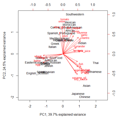
The figures look self-explanatory and does show the clustering together of geographically nearby regions on the basis of commonly used ingredients. Moreover, we also notice the grouping together of regions with historical travel patterns (North Europe and American, Spanish_Portuguese and SouthAmerican/Mexican) or historical trading patterns (Indian and Middle East).
We need to further test the stability of the grouping obtained here by including data from the Allrecipes dataset. Also, probably taking the third principal component might dissipate some of the crowd along the PC2 axis. These would be some of the tasks for the next post…
Here is the complete R code used for the analysis:
workdir <- "C:\Path\To\Dataset\Directory"
datafile <- file.path(workdir,"epic_recipes.txt")
data <- read.table(datafile, fill=TRUE, col.names=1:max(count.fields(datafile)),
na.strings=c("", "NA"), stringsAsFactors = FALSE)

a <- aggregate(data[,-1], by=list(data[,1]), paste, collapse=",")
a$combined <- apply(a[,2:ncol(a)], 1, paste, collapse=",")
a$combined <- gsub(",NA","",a$combined) ## this column contains the totality of all ingredients for a cuisine

cuisines <- as.data.frame(table(data[,1])) ## Number of recipes for each cuisine
freq <- lapply(lapply(strsplit(a$combined,","), table), as.data.frame) ## Frequency of ingredients
names(freq) <- a[,1]
prop <- lapply(seq_along(freq), function(i) {
colnames(freq[[i]])[2] <- names(freq)[i]
freq[[i]][,2] <- freq[[i]][,2]/cuisines[i,2] ## proportion (normalized frequency)
freq[[i]]}
)
names(prop) <- a[,1] ## this is a list of 26 elements, one for each cuisine

final <- Reduce(function(...) merge(..., all=TRUE, by="Var1"), prop)
row.names(final) <- final[,1]
final <- final[,-1]
final[is.na(final)] <- 0 ## If ingredient missing in all recipes, proportion set to zero
final <- t(final) ## proportion matrix

s <- sort(apply(final, 2, sd), decreasing=TRUE)
## Selecting ingredients with maximum variation in frequency among cuisines and
## Using standardized proportions for final analysis
final_imp <- scale(subset(final, select=names(which(s > 0.1))))

## heatmap
library(gplots)
heatmap.2(final_imp, trace="none", margins = c(6,11), col=topo.colors(7),
key=TRUE, key.title=NA, keysize=1.2, density.info="none")

## PCA and biplot
p <- princomp(final_imp)
biplot(p,pc.biplot=TRUE, col=c("black","red"), cex=c(0.9,0.8),
xlim=c(-2.5,2.5), xlab="PC1, 39.7% explained variance", ylab="PC2, 24.5% explained variance")

R-bloggers.com offers daily e-mail updates about R news and tutorials about learning R and many other topics. Click here if you're looking to post or find an R/data-science job.
Want to share your content on R-bloggers? click here if you have a blog, or here if you don't.