
24 Days of R: Day 9
Want to share your content on R-bloggers? click here if you have a blog, or here if you don't.
This will be the third time I've tried to write this post. I had started out presuming that I would uncover something fascinating about applying Bayesian inference to a low-frequency claims generation process. That isn't at all what I got and I ought to have known better when I started.
I started by doing very basic curve fitting presuming that I'm observing a Poisson process. I assume that the observations were losses excess of some monetary threshold. The overall number of losses is held constant. I'll produce 100 claims per year, every year. However, the average severity will change. For the first ten years, it's one number and then it drops meaningfully beginning with year 11. This will, of course, reduce the excess frequency. The excess point is set so that I expect roughly 5 claims per year. I'll then ensure that the reduced severity is such that the same excess will produce between 2 and 3 claims per year. (I did this through trial and error. It ought to be done with a bit more finesse.)
numClaims = 100
severity = 3500
# R uses 1 / mean for the exponential parameter. I'm going to call that
# theta and hope that no one (including me) gets confused by this.
theta = 1/severity
excess = qexp(0.95, theta)
excess = round(excess, -4)

theoreticalMean = numClaims * (1 - pexp(excess, theta))
years = 1:10
excessClaims = numeric(10)
set.seed(1234)
for (i in 1:10) {
    claims = rexp(numClaims, theta)
    excessClaims[i] = sum(claims > excess)
}

sampleMean = mean(excessClaims)
print(sampleMean)

## [1] 5.2

print(theoreticalMean)

## [1] 5.743

plot(excessClaims, pch = 19, xlab = "Year", ylab = "Excess claims")

In this case, the sample mean is not far off from the theoretical mean. If I could assume that the underlying parameters weren't changing (a very big if!) then I would feel comfortable using the sample mean to predict next year's claims. (Here, I'm assuming that we have no knowledge of the underlying claims. This would be the case if we were writing umbrella over another carrier's primary policy.)
I follow the example in Jim Albert's Bayesian Computation with R, which means that I'll assume the prior density is a gamma distribution. What does that mean our view of lambda is after two years? After five years? After ten?
x = seq(from = 0, to = 10, length.out = 250)

# We do this in reverse order because the density after ten years will have
# the largest values.
yTwo = dgamma(x, shape = sum(excessClaims[1:2]), rate = 2)
yFive = dgamma(x, shape = sum(excessClaims[1:5]), rate = 5)
yTen = dgamma(x, shape = sum(excessClaims[1:10]), rate = 10)

plot(x, yTen, type = "l", lwd = 3, xlab = "lambda", ylab = "Pr(lambda)")
lines(x, yFive, lwd = 2)
lines(x, yTwo, lwd = 1)

Over time, our confidence in the parameter grows and settles around 5.5 (roughly) which is close to the true mean. After ten years, we're fairly certain that lambda is nowhere near 8, for example. Now what happens when the underlying severity drops and the excess frequency plummets?
severity2 = 1750
theta2 = 1/severity2

years = 10:15
for (i in 10:15) {
    claims = rexp(numClaims, theta2)
    excessClaims[i] = sum(claims > excess)
}

theoreticalMean2 = numClaims * (1 - pexp(excess, theta2))
sampleMean2 = mean(excessClaims[11:15])

plot(excessClaims, pch = 19, xlab = "Year", ylab = "Excess claims")

For the most recent five years, our sample mean lines up well with the theoretical. But if we're pricing insurance in year 11, we don't know that at all. At that time, all that we can see is zero claims last year and one claim this year. In fact, we see (for this random sample) fewer than five claims per year for years 8 through 11. Four years is an eternity in the commercial insurance marketplace and I guarantee that there would be plenty of folks eager to talk about the improvement in claims results which began in year 8. That the Bayesian approach does not embrace this is a good thing. But it misses the drop in year 11.
How do things look after five years? That depends on how many years we use in our average. If we use all years- which is a good thing if the parameters don't change- then our sample mean is badly out of step with reality. We'll draw a distribution around lambda using all years and also show lambda after ten for comparison.
yFifteen = dgamma(x, shape = sum(excessClaims[1:15]), rate = 15)
plot(x, yFifteen, type = "l", lwd = 4, xlab = "lambda", ylab = "Pr(lambda)")
lines(x, yTen, lwd = 3)
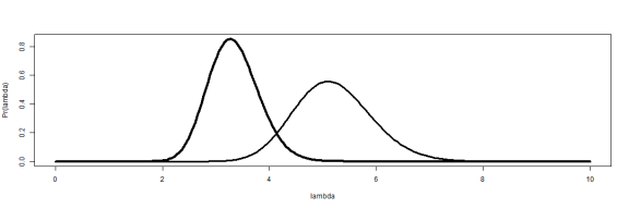
sample15 = mean(excessClaims[1:15])
There's a clear downward shift in response to the reduced number of claims. But it isn't enough. The full year sample is about 3.3, but next years claims will have a frequency of 0.33. A misestimation of that magnitude is deadly.
However, there is a bit more to this. What is the probability that the estimated lambda would produce the number of claims we saw in year 11? In year 12?
dpois(excessClaims[11], mean(excessClaims[1:11]))

## [1] 0.05179

dpois(excessClaims[12], mean(excessClaims[1:12]))

## [1] 0.01685
Not so good. This should make us question the use of all years in forming the estimate of claim frequency.
I know what you're thinking. There are any number of adjunct sources of information to incorporate. And perhaps that's the point. You also think that the example is a bit contrived. It's unlikely that an umbrella provider would have no view of the average claim size of underlying severities. True, but there are other rare phenomena with changing parameters: hurricanes, terrorist attacks, rare illnesses. I have a few more thoughts on this subject- I have a lot more thoughts on this subject- but they'll have to wait.
Tomorrow: if all goes well, more on Michael Caine.
sessionInfo()

## R version 3.0.2 (2013-09-25)
## Platform: x86_64-w64-mingw32/x64 (64-bit)
##
## locale:
## [1] LC_COLLATE=English_United States.1252
## [2] LC_CTYPE=English_United States.1252
## [3] LC_MONETARY=English_United States.1252
## [4] LC_NUMERIC=C
## [5] LC_TIME=English_United States.1252
##
## attached base packages:
## [1] stats     graphics  grDevices utils     datasets  methods   base
##
## other attached packages:
## [1] knitr_1.4.1      RWordPress_0.2-3
##
## loaded via a namespace (and not attached):
## [1] digest_0.6.3   evaluate_0.4.7 formatR_0.9    RCurl_1.95-4.1
## [5] stringr_0.6.2  tools_3.0.2    XML_3.98-1.1   XMLRPC_0.3-0

R-bloggers.com offers daily e-mail updates about R news and tutorials about learning R and many other topics. Click here if you're looking to post or find an R/data-science job.
Want to share your content on R-bloggers? click here if you have a blog, or here if you don't.