The implied option volatility reflects the price premium an option commands. A trader’s profit and loss ‘P&L’ from hedging option positions is driven to a large extend by the actual historical volatility of the underlying assets. Thus as option premiums are driven by supply and demand they should reflect to some extend the expectation of future realized asset volatility by market participants.

Bloomberg GV function displays option implied vs. realized volatility. Below for example for the Dow Jones INDU index both realized and implied volatility measures are reasonably aligned

Another interesting aspect in the context of dispersion trading is implied correlation. Implied correlation is a measure on how index volatility compares to the volatility of a basket of the individual index components. A trader can take a position in correlation for example by selling options of the individual component stocks and buying index options. Instead of taking position in options a similar strategy can also be executed using variance swaps.

The Dow Jones index I is comprised of 30 individual stocks S_i

with basket weights w_i.
The price volatility of the index is determined by the aggregation of individual stock volatilities according to its correlation structure. Let’s consider two extreme cases. In the situation the movement of all basket components are aligned the pairwise correlation between assets is 1. The correlation 1 basket variance V₁ is given by the squared sum of weighted asset volatilities

In case all asset movement disperse independent of each other the pairwise correlation between assets is 0. The correlation 0 basket variance V₀ is given by the sum of variances

The relation of the actual index variance V_I to these extreme cases is reflected by the implied correlation ρ

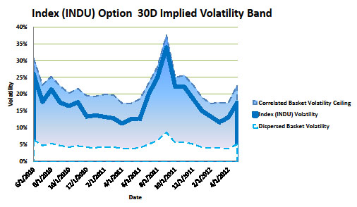
The graph below depicts the Dow Jones index implied volatility in the band between the dispersed correlation zero and extreme aligned correlation one cases.

The implied volatility is close to the upper range, indicating a high implied correlation. Plotting implied correlation directly confirms this

The graphs above are generated by downloading historical index and stock option implied volatility data into Excel using the Bloomberg specific functions,

=BDS(IndexTicker,"INDX_MWEIGHT","cols=2;rows=30")
=BDH("AA US EQUITY","PX_LAST",DATE(2010,6,30),DATE(2010,6,30)) 
=BDH("AA US EQUITY","30DAY_IMPVOL_100.0%MNY_DF",DATE(2010,6,30),DATE(2010,6,30))

for index composition, prices and implied option volatilities.

For calculation on the static data refer to the following google-docs spreadsheet, for better visibility right click the below and select ‘Open Frame in New Window’.

Finally let’s look at volatilities and correlations from raw realized asset prices

retrieved using the tawny and quantmod R packages

require(tawny)
indx <- getIndexComposition('^DJI')
for(stk in indx) { getSymbols(stk) }

widthNrBusDays <- 90
dayBasis <- 260
indx.ts <- xts()
var0.ts <- xts()
var1.ts <- xts()
divisor <- 0.13213
for(stk in indx) 
{
 	stk.ts<-Cl(get(stk)['2008-01::'])
        var.ts=apply.rolling(diff(log(stk.ts)),width=widthNrBusDays,FUN="var")*dayBasis
if(length(indx.ts) == 0)
{
        indx.ts <- stk.ts/divisor
        var0.ts <- var.ts*(stk.ts/divisor)^2
        var1.ts <- sqrt(var.ts)*stk.ts/divisor
} else {
       indx.ts = indx.ts + stk.ts/divisor
       var0.ts = var0.ts + var.ts*(stk.ts/divisor)^2
       var1.ts = var1.ts + sqrt(var.ts)*stk.ts/divisor
}
}
var0.ts = var0.ts/(indx.ts*indx.ts)
var1.ts = (var1.ts/indx.ts)^2

indx.var.ts <- apply.rolling(diff(log(indx.ts)),width=widthNrBusDays,FUN="var")*dayBasis

indx.corr.ts <- (indx.var.ts - var0.ts)/(var1.ts - var0.ts)
indx.vol.ts <-  sqrt(indx.var.ts)

par(mfrow=c(2,1))
chart_Series(indx.corr.ts, name='DJI 30 day implied correlation')
chart_Series(indx.vol.ts, name='DJI 30 day realized volatility')