
Visualizing and wrangling MCMC output in R with `MCMCvis`
Want to share your content on R-bloggers? click here if you have a blog, or here if you don't.
Model results can be thought of as a reward for the many hours of model design, troubleshooting, re-design, etc. that analyses often require. Following the potentially exhausting mental exercise to acquire these results, I think we’d all like the interpretation to be as straightforward as possible. Analyzing MCMC output from Bayesian analyses, which may include hundreds of parameters and/or derived quantities, however can often require a fair amount of code and (more importantly) time.
The MCMCvis package was designed to alleviate this problem, and streamline the analysis of Bayesian model results. The latest version (0.7.1) is now available on CRAN with bug fixes, speed improvements, and added functionality.
Why MCMCvis?
Using MCMCvis provides three principal benefits:
1) MCMC output fit with Stan, JAGS, or other MCMC samplers can be fed into all package functions as an argument with no further manipulation needed. No need to specify the type of object or how it was fit; the package does all of that behind the scenes.
2) Specific parameters or derived quantities of interest can be specified within each function, to avoid additional steps of data processing. This works using a grep like call for optimal efficiency.
3) The package creates ‘publication-ready’ posterior estimate visualizations (below). Parameters can now be plotted vertically or horizontally.
The package has four functions for basic MCMC output tasks:
MCMCsummary – summarize MCMC output for particular parameters of interest
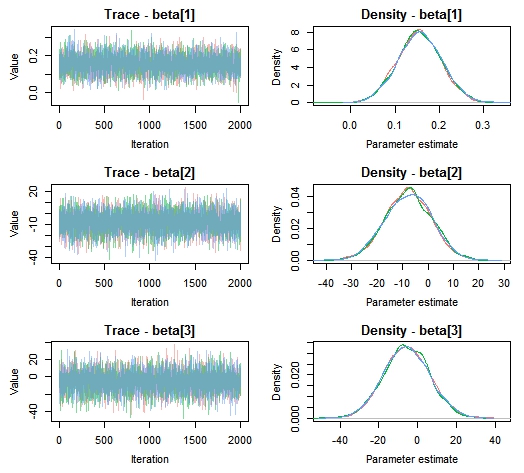
MCMCtrace – create trace and density plots of MCMC chains for particular parameters of interest
MCMCchains – easily extract posterior chains from MCMC output for particular parameters of interest
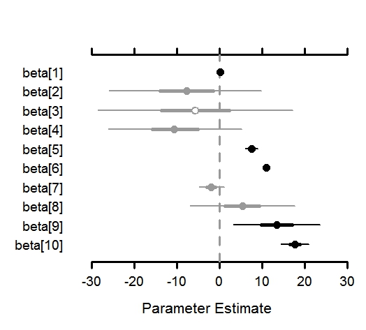
MCMCplot – create caterpillar plots from MCMC output for particular parameters of interest
The vignette can be found here.
An example workflow may go as follows:
– summarize posterior estimates for just beta parameters
#install package
install.packages('MCMCvis')

#load package
require(MCMCvis)

#load example data
data(MCMC_data)

#run summary function
MCMCsummary(MCMC_data,
             params = 'beta')

##            mean   2.5%    50% 97.5% Rhat
## beta[1]    0.16   0.06   0.15  0.25    1
## beta[2]   -7.77 -25.82  -7.68  9.78    1
## beta[3]   -5.64 -28.53  -5.76 17.23    1
## beta[4]  -10.39 -25.98 -10.63  5.27    1
## beta[5]    7.52   6.03   7.52  9.05    1
## beta[6]   10.89  10.10  10.89 11.68    1
## beta[7]   -1.91  -4.83  -1.92  1.08    1
## beta[8]    5.38  -6.86   5.45 17.67    1
## beta[9]   13.39   3.28  13.38 23.60    1
## beta[10]  17.63  14.41  17.63 20.86    1
– check posteriors for convergence
MCMCtrace(MCMC_data,
           params = c('beta[1]', 'beta[2]', 'beta[3]'),
           ind = TRUE)
– extract chains for beta parameters so that they can be manipulated directly
ex <- MCMCchains(MCMC_data, params = 'beta')
#find 22nd quantile for all beta parameters
apply(ex, 2, function(x){round(quantile(x, probs = 0.22), digits = 2)})

##  beta[1]  beta[2]  beta[3]  beta[4]  beta[5]  beta[6]  beta[7]  beta[8]  beta[9] beta[10]
##    0.12   -14.86   -14.80   -16.48     6.91    10.58    -3.09     0.68     9.29    16.36
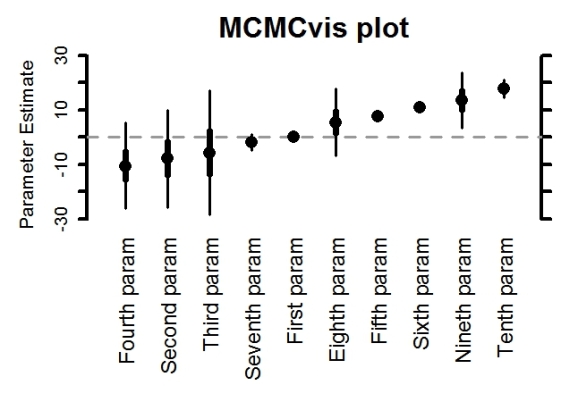
– create caterpillar plots for posterior estimates. Shading represents whether 50% CI (gray with open circle), 95% CI (gray with closed circle), or neither (black) overlap 0. This option can be turned off (as below). A variety of options exist, including the ability to plot posteriors vertically rather than horizontally
MCMCplot(MCMC_data,
          params = 'beta',
          horiz = FALSE,
          rank = TRUE,
          ref_ovl = FALSE,
          xlab = 'My x-axis label',
          main = 'MCMCvis plot',
          labels = c('First param', 'Second param', 'Third param',
          'Fourth param', 'Fifth param', 'Sixth param', 'Seventh param',
          'Eighth param', 'Nineth param', 'Tenth param'),
          labels_sz = 1.5, med_sz = 2, thick_sz = 7, thin_sz = 3,
          ax_sz = 4, main_text_sz = 2)
Follow Casey Youngflesh on Twitter @caseyyoungflesh. The MCMCvis source code can be found on GitHub.
R-bloggers.com offers daily e-mail updates about R news and tutorials about learning R and many other topics. Click here if you're looking to post or find an R/data-science job.
Want to share your content on R-bloggers? click here if you have a blog, or here if you don't.