[This article was first published on DataGeeek, and kindly contributed to R-bloggers]. (You can report issue about the content on this page here)
Want to share your content on R-bloggers? click here if you have a blog, or here if you don't.
In Turkey, some parts of society always compare Turkey to Germany and think that we are better than Germany for a lot of issues. The same applies to COVID-19 crisis management; is that reflects to true?
We will use two variables for compared parameters; the number of daily new cases and daily new deaths.First, we will compare the mean of new cases of the two countries. The dataset we’re going to use is here.
#load and tidying the dataset
library(readxl)
deu <- read_excel("covid-data.xlsx",sheet = "deu")
deu$date <- as.Date(deu$date)
tur <- read_excel("covid-data.xlsx",sheet = "tur")
tur$date <- as.Date(tur$date)
#building the function comparing means on grid table
grid_comparing <- function(column="new_cases"){
table <-data.frame(
deu=c(mean=mean(deu[[column]]),sd=sd(deu[[column]]),n=nrow(deu)),
tur=c(mean=mean(tur[[column]]),sd=sd(tur[[column]]),n=nrow(tur))
) %>% round(2)
grid.table(table)
}
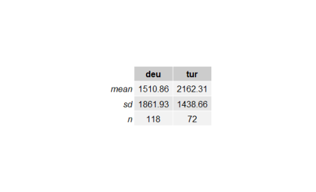
grid_comparing()
Above table shows that the mean of new cases in Turkey is greater than Germany. To check it, we will inference concerning the difference between two means.
In order to make statistical inference for the , the sample distribution must be approximately normal distribution. If it is assumed that the related populations will not be normal, sample distribution is approximately normal only in the volume of relevant samples greater than 30 separately according to the central limit theorem. In this case, the distribution is assumed approximately normal.
If the variances of two populations and are known, z-distribution would be used for statistical inference. A more common situation, if the variances of population are unknown, we will instead use samples variances , and distribution.
When and are unknown, two situation are examined.
: the assumption they are equal.
: the assumption they are not equal.
There is a formal test to check whether population variances are equal or not which is a hypothesis test for the ratio of two population variances. A two-tailed hypothesis test is used for this as shown below.
The test statistic for :
The sample volumes and , degrees of freedom of the samples and . F-distribution is used to describe the sample distribution of
var.test(deu$new_cases,tur$new_cases)

#	F test to compare two variances

#data:  deu$new_cases and tur$new_cases
#F = 1.675, num df = 117, denom df = 71, p-value = 0.01933
#alternative hypothesis: true ratio of variances is not equal to 1
#95 percent confidence interval:
# 1.088810 2.521096
#sample estimates:
#ratio of variances
#          1.674964
At the %5 significance level, because p-value(0.01933) is less than 0.05, the null hypothesis() is rejected and we assume that variances of the populations are not equal.
Because the variances are not equal we use Welch’s t-test to calculate test statistic:
The degree of freedom:
Let’s see whether the mean of new cases per day of Turkey() greater than Germany(); to do that we will build the hypothesis test as shown below:


}=")


} {\sqrt{(\frac{s_1^2} {n_1}+\frac{s_2^2} {n_2})}}")
^2} {(s_1^2/n_1)^2/(n_1-1)+(s_2^2/n_2)^2/(n_2-1)}")


