
The tidy caret interface in R
Want to share your content on R-bloggers? click here if you have a blog, or here if you don't.

Among most popular off-the-shelf machine learning packages available to R, caret ought to stand out for its consistency. It reaches out to a wide range of dependencies that deploy and support model building using a uniform, simple syntax. I have been using caret extensively for the past three years, with a precious partial least squares (PLS) tutorial in my track record.
A couple of years ago, the creator and maintainer of caret Max Kuhn joined RStudio where he has contributing new packages to the ongoing tidy-paranoia – the supporting recipes, yardstick, rsample and many other packages that are part of the tidyverse paradigm and I knew little about. As it happens, caret is now best used with some of these. As an aspiring data scientist with fashionable hex-stickers on my laptop cover and a tendency to start any sentence with ‘big data’, I set to learn tidyverse and going Super Mario using pipes (%>%, Ctrl + Shift + M).
Overall, I found the ‘tidy’ approach quite enjoyable and efficient. Besides streamlining model design in a sequential manner, recipes and the accompanying ‘tidy’ packages fix a common problem in the statistical learning realm that curtails predictive accuracy, data leakage. You can now generate a ‘recipe’ that lays out the plan for all the feature engineering (or data pre-processing, depending on how many hex-stickers you have) and execute it separately for validation and resampling splits (i.e. split first, process later), thus providing a more robust validation scheme. It also enables recycling any previous computations afterwards.
I drew a lot of inspiration from a webinar and a presentation from Max himself to come up with this tutorial. Max is now hands-on writing a new book, entitled Feature Engineering and Selection: A Practical Approach for Predictive Models that will include applications of caret supported by recipes. I very much look forward to read it considering he did a fantastic job with Applied Predictive Modeling.
The aim here is to test this new caret framework on the DREAM Olfaction Prediction Challenge, a crowd-sourced initiative launched in January 2015. This challenge demonstrated predictive models can identify perceptual attributes (e.g. coffee-like, spicy and sweet notes) in a collection of fragrant compounds from physicochemical features (e.g. atom types). Results and conclusions were condensed into a research article [1] that reports an impressive predictive accuracy for a large number of models and teams, over various perceptive attributes. Perhaps more impressive yet, is the fact it anticipates the very scarce knowledge of human odour receptors and their molecular activation mechanisms. Our task, more concretely, will be to predict population-level pleasantness of hundreds of compounds from physicochemical features, using the training set of the competition.
Finally, a short announcement. Many people have been raising reproducibility issues with previous entries, due to either package archiving (e.g. GenABEL, for genetic mapping) or cross-incompatibility (e.g. caret, for PLS). There were easy fixes for the most part, but I have nevertheless decided to start packing scripts together with sessionInfo() reports in unique GitHub repositories. The bundle for this tutorial is available under https://github.com/monogenea/olfactionPrediction. I hope this will help track down the exact package versions and system configurations I use, so that anyone can anytime fully reproduce these results. No hex-stickers required!
NOTE that most code chunks containing pipes are corrupted. PLEASE refer to the materials from the repo.
The DREAM Olfaction Prediction Challenge
The DREAM Olfaction Prediction Challenge training set consists of 338 compounds characterised by 4,884 physicochemical features (the design matrix), and profiled by 49 subjects with respect to 19 semantic descriptors, such as ‘flower’, ‘sweet’ and ‘garlic’, together with intensity and pleasantness (all perceptual attributes). Two different dilutions were used per compound. The perceptual attributes were given scores in the 0-100 range. The two major goals of the competition were to use the physicochemical features in modelling i) the perceptual attributes at the subject-level and ii) both the mean and standard deviation of the perceptual attributes at the population-level. How ingenious it was to model the standard deviation, the variability in how something tastes to different people! In the end, the organisers garnered important insights about the biochemical basis of flavour, from teams all over the world. The resulting models were additionally used to reverse-engineer nonexistent compounds from target sensory profiles – an economically exciting prospect.
According to the publication, the top-five best predicted perceptual attributes at the population-level (i.e. mean values across all 49 subjects) were ‘garlic’, ‘fish’, ‘intensity’, pleasantness and ‘sweet’ (cf. Fig. 3A in [1]), all exhibiting average prediction correlations of 
Since pleasantness is one of the most general olfactory properties, I propose modelling the population-level median pleasantness of all compounds, from all physicochemical features. The median, as opposed to the mean, is less sensitive to outliers and an interesting departure from the original approach we can later compare against.
Let’s get started with R
We can start off by loading all the necessary packages and pulling the data directly from the DREAM Olfaction Prediction GitHub repository. More specifically, we will create a directory called data and import both the profiled perceptual attributes (TrainSet.txt) and the physicochemical features that comprise our design matrix (molecular_descriptors_data.txt). Because we are tidy people, we will use readr to parse these as tab-separated values (TSV). I also suggest re-writing the column name Compound Identifier in the sensory profiles into CID, to match with that from the design matrix molFeats.
# Mon Oct 29 13:17:55 2018 ------------------------------
## DREAM olfaction prediction challenge
library(caret)
library(rsample)
library(tidyverse)
library(recipes)
library(magrittr)
library(doMC)

# Create directory and download files
dir.create("data/")
ghurl <- "https://github.com/dream-olfaction/olfaction-prediction/raw/master/data/"
download.file(paste0(ghurl, "TrainSet.txt"),
destfile = "data/trainSet.txt")
download.file(paste0(ghurl, "molecular_descriptors_data.txt"),
destfile = "data/molFeats.txt")

# Read files with readr, select least diluted compounds
responses %
rename(CID = `Compound Identifier`)

molFeats <- read_tsv("data/molFeats.txt") # molecular features
Next, we filter compounds that are common to both datasets and reorder them accordingly. The profiled perceptual attributes span a total of 49 subjects, two different dilutions and some replications (cf. Fig. 1A in [1]). Determine the median pleasantness (i.e. VALENCE/PLEASANTNESS) per compound, across all subjects and dilutions while ignoring missingness with na.rm = T. The last line will ensure the order of the compounds is identical between this new dataset and the design matrix, so that we can subsequently introduce population-level pleasantness as a new column termed Y in the new design matrix X. We no longer need CID so we can discard it.
Regarding missingness, I found maxima of 0.006% and 23% NA content over all columns and rows, respectively. A couple of compounds could be excluded but I would move on.
# Determine intersection of compounds in features and responses
commonMols %
dplyr::summarise(pleasantness = median(`VALENCE/PLEASANTNESS`, na.rm = T))
all(medianPlsnt$CID == molFeats$CID) # TRUE - rownames match

# Concatenate predictors (molFeats) and population pleasantness
X %
select(-CID)
In examining the structure of the design matrix, you will see there are many skewed binary variables. In the most extreme case, if a binary predictor is either all zeros or all ones throughout it is said to be a zero-variance predictor that if anything, will harm the model training process. There is still the risk of having near-zero-variance predictors, which can be controlled based on various criteria (e.g. number of samples, size of splits). Of course, this can also impact quantitative, continuous variables. Here we will use nearZeroVar from caret to identify faulty predictors that are either zero-variance or display values whose frequency exceeds a predefined threshold. Having a 5x repeated 5-fold cross-validation in mind, I suggest setting freqCut = 4, which will rule out i) binary variables with  - f(1)| \ge 0.80")

?nearZeroVar for more information. From 4,870 features we are left with 2,554 – a massive reduction by almost a half.
# Filter nzv
X <- X[,-nearZeroVar(X, freqCut = 4)] # == 80/20
Now we will use rsample to define the train-test and cross-validation splits. Please use set.seed as it is, to ensure you will generate the same partitions and arrive to the same results. Here I have allocated 10% of the data to the test set; by additionally requesting stratification based on the target Y, we are sure to have a representative subset. We can next pass the new objects to training and testing to effectively split the design matrix into train and test sets, respectively. The following steps consist of setting up a 5x repeated 5-fold cross-validation for the training set. Use vfold_cv and convert the output to a caret-like object via rsample2caret. Next, initialise a trainControl object and overwrite index and indexOut using the corresponding elements in the newly converted vfold_cv output.
# Split train/test with rsample
set.seed(100)
initSplit <- initial_split(X, prop = .9,
strata = "Y")
trainSet <- training(initSplit)
testSet <- testing(initSplit)

# Create 5-fold cross-validation, convert to caret class
set.seed(100)
myFolds %
rsample2caret()
ctrl <- trainControl(method = "cv",
selectionFunction = "oneSE")
ctrl$index <- myFolds$index
ctrl$indexOut <- myFolds$indexOut
Prior to modelling, I will create two reference variables – binVars, to identify binary variables, and missingVars, to identify any variables containing missing values. These will help with i) excluding binary variables from mean-centering and unit-variance scaling, and ii) restricting mean-based imputation to variables that do contain missing values, respectively.
# binary vars
binVars <- which(sapply(X, function(x){all(x %in% 0:1)}))
missingVars <- which(apply(X, 2, function(k){any(is.na(k))}))
Recipes are very simple in design. The call to recipe is first given the data it is supposed to be applied on, as well as a lm-style formula. The recipes package contains a family of functions with a step_... prefix, involved in encodings, date conversions, filters, imputation, normalisation, dimension reduction and a lot more. These can be linked using pipes, forming a logic sequence of operations that starts with the recipe call. Supporting functions such as all_predictors, all_outcomes and all_nominal delineate specific groups of variables at any stage in the sequence. One can also use the names of the variables, akin to my usage of binVars and missingVars.
I propose writing a basic recipe myRep that does the following:
- Yeo-Johnson [2] transformation of all quantitative predictors;
- Mean-center all quantitative predictors;
- Unit-variance scale all quantitative predictors;
- Impute missing values with the mean of the incident variables.
# Design recipe
myRec %
step_YeoJohnson(all_predictors(), -binVars) %>%
step_center(all_predictors(), -binVars) %>%
step_scale(all_predictors(), -binVars) %>%
step_meanimpute(missingVars)
In brief, the Yeo-Johnson procedure transforms variables to be distributed as Gaussian-like as possible. Before delving into the models let us tweak the recipe and assign it to pcaRep, conduct a principal component analysis and examine how different compounds distribute along the first two principal components. Colour them based on their population-level pleasantness – red for very pleasant, blue for very unpleasant and the gradient in between, via colGrad.
# simple PCA, plot
pcaRec %
step_pca(all_predictors())

myPCA %
juice()
colGrad <- trainSet$Y/100 # add color

plot(myPCA$PC1, myPCA$PC2,
col = rgb(1 - colGrad, 0, colGrad,.5),
pch = 16, xlab = "PC1", ylab = "PC2")
legend("topleft", pch = 16,
col = rgb(c(0,.5,1), 0, c(1,.5,0), alpha = .5),
legend = c("Pleasant", "Neutral", "Unpleasant"), bty = "n")
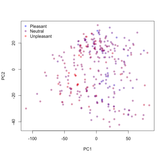
The compounds do not seem to cluster into groups, nor do they clearly separate with respect to pleasantness.
Note that pcaRep itself is just a recipe on wait. Except for recipes passed to caret::train, to process and extract the data as instructed you need to either ‘bake’ or ‘juice’ the recipe. The difference between the two is that ‘juicing’ outputs the data associated to the recipe (e.g. the training set), whereas ‘baking’ can be applied to process any other dataset. ‘Baking’ is done with bake, provided the recipe was trained using prep. I hope this explains why I used juice above!
Next we have the model training. I propose training five regression models – k-nearest neighbours (KNN), elastic net (ENET), support vector machine with a radial basis function kernel (SVM), random forests (RF), extreme gradient boosting (XGB) and Quinlan’s Cubist (CUB) – aiming at minimising the root mean squared error (RMSE). Note I am using tuneGrid and tuneLength interchangeably. I rather supply predefined hyper-parameters to simple models I am more familiar with, and run the rest with a number of defaults via tuneLength.
Parallelise the computations if possible. With macOS, I can use registerDoMC from the doMC package to harness multi-threading of the training procedure. If you are running a different OS, please use a different library if necessary. To the best of my knowledge, doMC will also work in Linux but Windows users might need to use the doParallel package instead.
# Train
doMC::registerDoMC(10)
knnMod <- train(myRec, data = trainSet,
method = "knn",
tuneGrid = data.frame(k = seq(5, 25, by = 4)),
trControl = ctrl)

enetMod <- train(myRec, data = trainSet,
method = "glmnet",
tuneGrid = expand.grid(alpha = seq(0, 1, length.out = 5),
lambda = seq(.5, 2, length.out = 5)),
trControl = ctrl)

svmMod <- train(myRec, data = trainSet,
method = "svmRadial",
tuneLength = 8,
trControl = ctrl)

rfMod <- train(myRec, data = trainSet,
method = "ranger",
tuneLength = 8,
num.trees = 5000,
trControl = ctrl)

xgbMod <- train(myRec, data = trainSet,
method = "xgbTree",
tuneLength = 8,
trControl = ctrl)

cubMod <- train(myRec, data = trainSet,
method = "cubist",
tuneLength = 8,
trControl = ctrl)

modelList <- list("KNN" = knnMod,
"ENET" = enetMod,
"SVM" = svmMod,
"RF" = rfMod,
"XGB" = xgbMod,
"CUB" = cubMod)
Once the training is over, we can compare the optimal five cross-validated models based on their RMSE across all 
bwplot magic sponsored by lattice. In my case the runtime was unusually long (>2 hours) compared to previous releases.
bwplot(resamples(modelList),
metric = "RMSE")

The cross-validated RSME does not vary considerably across the six optimal models. To conclude, I propose creating a model ensemble by simply taking the average predictions of all six optimal models on the test set, to compare observed and predicted population-level pleasantness in this hold-out subset of compounds.
# Validate on test set with ensemble
allPreds <- sapply(modelList, predict, newdata = testSet)
ensemblePred <- rowSums(allPreds) / length(modelList)

# Plot predicted vs. observed; create PNG
plot(ensemblePred, testSet$Y,
xlim = c(0,100), ylim = c(0,100),
xlab = "Predicted", ylab = "Observed",
pch = 16, col = rgb(0, 0, 0, .25))
abline(a=0, b=1)

writeLines(capture.output(sessionInfo()), "sessionInfo")

The ensemble fit on the test set is not terrible – slightly underfit, predicting the poorest in the two extremes of the pleasantness range. All in all, it attained a prediction correlation of 
Wrap-up
The revamped caret framework is still under development, but it seems to offer
- A substantially expanded, unified syntax for models and utils. Keep an eye on
textrecipes, an upcoming complementary package for processing textual data; - A sequential streamlining of extraction, processing and modelling, enabling recycling of previous computations;
- Executing-after-splitting, thereby precluding leaky validation strategies.
On the other hand, I hope to see improvements in
- Decoupling from proprietary frameworks in the likes of
tidyverse, although there are alternatives; - The runtime. I suspect the recipes themselves are the culprit, not the models. Future updates will certainly fix this.
Regarding the DREAM Olfaction Prediction Challenge, we were able to predict population-level perceived pleasantness from physicochemical features with an accuracy as good as that achieved, in average, by the competing teams. Our model ensemble seems underfit, judging from the narrow range of predicted values. Maybe we could be less restrictive about the near-zero-variance predictors and use a repeated 3-fold cross-validation.
I hope you had as much fun as I did in dissecting a fascinating problem while unveiling a bit of the new caret. You can use this code as a template for exploring different recipes and models. If you encounter any problems or have any questions do not hesitate to post a comment underneath – we all learn from each other!
References
[1] Keller, Andreas et al. (2017). Predicting human olfactory perception from chemical features of odor molecules. Science, 355(6327), 820-826.
[2] Yeo, In-Kwon and Johnson, Richard (2000). A new family of power transformations to improve normality or symmetry. Biometrika, 87(4), 954-959.
R-bloggers.com offers daily e-mail updates about R news and tutorials about learning R and many other topics. Click here if you're looking to post or find an R/data-science job.
Want to share your content on R-bloggers? click here if you have a blog, or here if you don't.