Autocorrelation of a time series can be useful for prediction because the most recent observation of the prediction target contains information about future values. At the same time autocorrelation can play tricks on you because many standard statistical methods implicitely assume independence of measurements at different times.

The correlation coefficient between two variable and has expectation value zero if two variables are statistically independent of each other. However, if calculated from a finite sample of the two variables, the correlation coefficient might be spuriously different from zero. The magnitude of such spurious correlation coefficients increases if the variables are autocorrelated, as shown by this plot:

R code:

N <- 150
K <- 1000
cc1 <- vector()
cc2 <- vector()
cc3 <- vector()
#calculate K corr. coeffs for each process
for (k in seq(K)) {
    #white noise
    x <- rnorm(N)
    y <- rnorm(N)
    cc1 <- rbind(cc1,cor(x,y))
    #AR 1
    x <- arima.sim(model=list(order=c(1,0,0),ar=0.5),n=N)
    y <- arima.sim(model=list(order=c(1,0,0),ar=0.5),n=N)
    cc2 <- rbind(cc2,cor(x,y))
    #random walk
    x <- cumsum(rnorm(N))
    y <- cumsum(rnorm(N))
    cc3 <- rbind(cc3,cor(x,y))
}
#plot corr coeff histograms
jpeg("cc-hist.jpg",width=400,height=700,quality=100)
par(mar=c(5,5,5,2),cex.axis=2,cex.lab=2,cex.main=2)
layout(seq(3))
hist(cc1,breaks=seq(-1,1,.1),main="white noise",xlab="")
hist(cc2,breaks=seq(-1,1,.1),main="AR(1)",xlab="")
hist(cc3,breaks=seq(-1,1,.1),main="random walk",xlab="corr. coeff.")
dev.off()

For the above plot, correlation coefficients were calculated between realizations of white noise, of autoregressive first order processes (), and of random walks. The lengths of the time series is 150 and 1000 correlation coefficients were calculated for ach process.

Here are examples of the three processes:

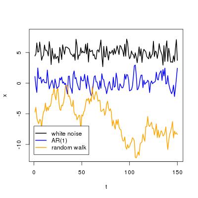
For white noise, the histogram over the observed correlation coefficients is sharply peaked around zero. In most cases, the correlation coefficient is very close to zero. Its absolute value rarely exceeds 0.25. For the AR(1) process, the histogram looks similar, however, more coefficients larger than 0.1 are observed than for white noise. In the case of random walk, the picture changes completely. You are equally likely to observe a coefficient between 0 and 0.1 and between 0.7 and 0.8, even though the processes are completely independent from each other. The probability of observing spurious correlation increases if the variables are autocorrelated.

The lasso is a popular statistical method for constructing prediction models for a target , based on linear superposition of inputs . That is, the lasso is a method to find “good” coefficients for the model

One of the great strengths of the lasso is that it can detect inputs which contain no information about the target . The lasso sets the corresponding to exactly zero. This property makes the lasso a workhorse of statistical modeling because it can produce parsimonious models if many potential predictors are available. In R, the packages glmnet contains an efficient implementation of the lasso. If the variable Y is the target and the variable X is the matrix of inputs, which satisfies length(Y)=dim(X)[1], a lasso model can be fit by

lasso.model <- cv.glmnet(x=X,y=Y)

and the coefficient vector beta is extracted by

beta <- coef(lasso.model,s=lasso.model$lambda.min)

If there is no relation between Y and the columns of X, all elements of beta except the first one should be equal to zero. However, spurious correlation may lead to some of the coefficients being different from zero, thus suggesting that some of the inputs in X do contain some expalantory power with respect to Y. The lasso (at least its implementation in glmnet) is sensitive to such spurious correlations as the following histograms show

R code:

library(glmnet)
library(multicore)
N <- 150
M <- 50
K <- 500
#function that returns number of nonzero coefficients
#for three lasso models, (length N, number of regressors M),
#where x and y are white noise, AR1 processes, or random walks
#x and y are always unrelated
nlasso <- function(dummy) {
    #white noise target, white noise inputs
    x <- matrix(rnorm(N*M),ncol=M)
    y <- rnorm(N)
    m <- cv.glmnet(x=x,y=y)
    coefz <- coef(m,s=m$lambda.min)[-1]
    ncoef1 <- length(which(coefz!=0))
    #AR1 targets, AR1 inputs
    x <- lapply(seq(50),function(z) arima.sim(model=list(order=c(1,0,0),ar=.5),n=N))
    x <- apply(as.matrix(x),1,unlist)
    y <- as.vector( arima.sim(model=list(order=c(1,0,0),ar=.5),n=N) )
    m <- cv.glmnet(x=x,y=y)
    coefz <- coef(m,s=m$lambda.min)[-1]
    ncoef2 <- length(which(coefz!=0))
    #random walk target, random walk inputs
    x <- matrix(rnorm(N*M),ncol=M)
    x <- apply(x,2,cumsum)
    y <- cumsum(rnorm(N))
    m <- cv.glmnet(x=x,y=y)
    coefz <- coef(m,s=m$lambda.min)[-1]
    ncoef3 <- length(which(coefz!=0))
    #return
    c(ncoef1,ncoef2,ncoef3)
}
#get the numbers K times and calculate histograms
ncoef <- mclapply(seq(K),nlasso,mc.cores=8)
ncoef <- t(apply(as.matrix(ncoef),1,unlist))
h1 <- hist(ncoef[,1],breaks=seq(-.5,M+.5),plot=F)
h2 <- hist(ncoef[,2],breaks=seq(-.5,M+.5),plot=F)
h3 <- hist(ncoef[,3],breaks=seq(-.5,M+.5),plot=F)
#plot
jpeg("ncoef-hist.jpg",width=400,height=700,quality=100)
par(mar=c(5,5,5,2),cex.axis=2,cex.lab=2,cex.main=2)
layout(seq(3))
plot(seq(M+1),h1$counts,main="white noise",xlab="",ylab="Frequency",type="s")
plot(seq(M+1),h2$counts,main="AR(1)",xlab="",ylab="Frequency",type="s")
plot(seq(M+1),h3$counts,main="random walk",xlab="number of nonzero lasso coeffs.",ylab="Frequency",type="s")
dev.off()

The histograms give an idea of how many of the 50 possible coefficients are non-zero. Ideally, all coefficients should vanish because by construction there is no relation between inputs and target. In the case of indpendent white noise the lasso almost always sets them all to zero. Only on rare occasions does the number of nonzero coefficients exceed 5. In the case of AR(1) target and inputs, coefficient vectors beta with more than 20 nonzero coefficients occur quite frequently. This is even worse in the case of random walks. The smallest number of nonzero coefficients observed in 1000 experiments is 18! In some cases even 50 coefficients are nonzero, that is, the lasso assigns predictive skill to all 50 inputs, even though none of them has any relation to the target.

The effect will become weaker as the length of the time series increases. Furthermore, there might be implementations of the lasso that are able to take such spurious correlations into account. The bottom line is that in prediction problems autocorrelation can be useful but if it is ignored it can (and will) lead to dubious statistical models.