
Simulating local community dynamics under ecological drift
Want to share your content on R-bloggers? click here if you have a blog, or here if you don't.
In 2001 the book by Stephen Hubbell on the neutral theory of biodiversity was a major shift from classical community ecology. Before this book the niche-assembly framework was dominating the study of community dynamics. Very briefly under this framework local species composition is the result of the resource available at a particular site and species presence or absence depends on species niche (as defined in Chase 2003). As a result community assembly was seen as a deterministic process and a specific set of species should emerge from a given set of resources and species composition should be stable as long as the system is not disturbed. Hubbell theory based on a dispersal-assembly framework (historically developed by MacArthur and Wilson) was a departure from this mainstream view of community dynamics by assuming that local species composition are transient with the absence of any equilibrium. Species abundance follow a random walk under ecological drift, species are continuously going locally extinct while a constant rain of immigrants from the metacommunity bring new recruits. The interested reader is kindly encouraged to read: this, that or that.
Being an R geek and after reading Chapter 4 of Hubbell’s book, I decided to implement his model of local community dynamic under ecological drift. Do not expect any advanced analysis of the model behavior, Hubbell actually derive in this chapter analytical solutions for this model. This post is mostly educational to get a glimpse into the first part of Hubbell’s neutral model.
Before diving into the code it is helpful to verbally outline the main characteristics of the model:
- The model is individual-based and neutral, assuming that all individuals are equal in their probability to die or to persist.
- The model assume a zero-sum dynamic, the total number of individual (J) is constant, imagine for example a forest. When a tree dies it allows for a new individual to grow and use the free space
- At each time step a number of individual (D) dies and are replaced by new recruits coming either from the metacommunity (with probability m) or from the local communities (with probability 1-m)
- The species identity of the new recruit is proportional to the species relative abundance either in the metacommunity (assumed to be fixed and having a log-normal distribution) or in the local community (which obviously varies)
We are now equipped to immerse ourselves into R code:
#implement zero-sum dynamic with ecological drift from Hubbel theory (Chp4)
untb<-function(R=100,J=1000,D=1,m=0,Time=100,seed=as.numeric(Sys.time())){
  mat<-matrix(0,ncol=R,nrow=Time+1,dimnames=
  + list(paste0("Time",0:Time),as.character(1:R)))
  #the metacommunity SAD
  metaSAD<-rlnorm(n=R)
  metaSAD<-metaSAD/sum(metaSAD)
  #initialize the local community
  begin<-table(sample(x=1:R,size = J,replace = TRUE,prob = metaSAD))
  mat[1,attr(begin,"dimnames")[[1]]]<-begin
  #loop through the time and get community composition
  for(i in 2:(Time+1)){
    newC<-helper_untb(vec = mat[(i-1),],R = R,D = D,m = m,metaSAD=metaSAD)
    mat[i,attr(newC,"dimnames")[[1]]]<-newC
  }
  return(mat)
}
#the function that compute individual death and
#replacement by new recruits
helper_untb<-function(vec,R,D,m,metaSAD){
  ind<-rep(1:R,times=vec)
  #remove D individuals from the community
  ind_new<-ind[-sample(x = 1:length(ind),size = D,replace=FALSE)]
  #are the new recruit from the Local or Metacommunity?
  recruit<-sample(x=c("L","M"),size=D,replace=TRUE,prob=c((1-m),m))
  #sample species ID according to the relevant SAD
  ind_recruit<-c(ind_new,sapply(recruit,function(isLocal) {
    if(isLocal=="L")
      sample(x=ind_new,size=1)
    else
      sample(1:R,size=1,prob=metaSAD)
  }))
I always like simple theories that can be implemented with few lines of code and do not require fancy computations. Let’s put the function in action and get for a closed community (m=0) of 10 species the species abundance and the rank-abundance distribution dynamics:
library(reshape2) #for data manipulation I
library(plyr) #for data manipulation II
library(ggplot2) #for the nicest plot in the world
#look at population dynamics over time
comm1<-untb(R = 10,J = 100,D = 10,m = 0,Time = 200)
#quick and dirty first graphs
comm1m<-melt(comm1)
comm1m$Time<-as.numeric(comm1m$Var1)-1
ggplot(comm1m,aes(x=Time,y=value,color=factor(Var2)))
+geom_path()+labs(y="Species abundance")
+scale_color_discrete(name="Species ID")
#let's plot the RAD curve over time
pre_rad<-apply(comm1,1,function(x) sort(x,decreasing = TRUE))
pre_radm<-melt(pre_rad)
pre_radm$Time<-as.numeric(pre_radm$Var2)-1
ggplot(pre_radm,aes(x=Var1,y=value/100,color=Time,group=Time))
+geom_line()+labs(x="Species rank",y="Species relative abundance")

We see there an important feature of the zero-sum dynamics, with no immigration the model will always (eventually) lead to the dominance of one species. This is because with no immigration there are so-called absorbing states, species abundance are attracted to these states and once these values are reached species abundance stay constant. In this case there are only two absorbing states for species relative abundance: 0 or 1, either you go extinct or you dominate the community.
In the next step we open up the community while varying the death rate and we track species richness dynamic:
#apply this over a range of parameters
pars<-expand.grid(R=20,J=200,D=c(1,2,4,8,16,32,64),
 + m=c(0,0.01,0.05,0.1,0.5),Time=200)
comm_list<-alply(pars,1,function(p) do.call(untb,as.list(p)))
#get species abundance for each parameter set
rich<-llply(comm_list,function(x) apply(x,1,function(y) length(y[y!=0])))
rich<-llply(rich,function(x) data.frame(Time=0:200,Rich=x))
rich<-rbind.fill(rich)
rich$D<-rep(pars$D,each=201)
rich$m<-rep(pars$m,each=201)
ggplot(rich,aes(x=Time,y=Rich,color=factor(D)))+geom_path()
+facet_grid(.~m)
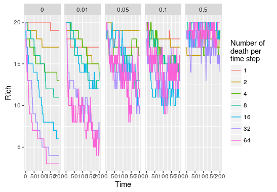
As we increase the probability that new recruit come from the metacommunity, the impact of increasing the number of death per time step becomes null. This is because the metacommunity is static in this model, even if species are wiped out by important local disturbance there will always be new immigrants coming in maintaining species richness to rather constant levels.
There is an R package for everything these days and the neutral theory is not an exception, check out the untb package which implement the full neutral model (ie with speciation and dynamic metacommunities) but also allow to fit the model to empirical data and to get model parameter estimate.
Filed under: Biological Stuff, R and Stat Tagged: Biodiversity, Neutral theory, R


R-bloggers.com offers daily e-mail updates about R news and tutorials about learning R and many other topics. Click here if you're looking to post or find an R/data-science job.
Want to share your content on R-bloggers? click here if you have a blog, or here if you don't.