
Sampling paths from a Gaussian process
Want to share your content on R-bloggers? click here if you have a blog, or here if you don't.
Gaussian processes are a widely employed statistical tool because of their flexibility and computational tractability. (For instance, one recent area where Gaussian processes are used is in machine learning for hyperparameter optimization.)
A stochastic process 
")

")

The stochastic nature of Gaussian processes also allows it to be thought of as a distribution over functions. One draw from a Gaussian process over corresponds to choosing a function 
Gaussian processes are defined by their mean and covariance functions. The covariance (or kernel) function 

(Click on this link to see all code for this post in one script. For more technical details on the covariance functions, see this previous post.)
Overall set-up
Let’s say we have a zero-centered Gaussian process denoted by , K(\cdot, \cdot))")

")
, \dots, f(x_n))")
, \dots, m(x_n))")

")
mvrnorm() from the MASS package to draw the function values at these points, then connect them with straight lines.
Assume that we have already written an R function kernel_fn for the kernel. The first function below generates a covariance matrix from this kernel, while the second takes N draws from this kernel (using the first function as a subroutine):
library(MASS)

# generate covariance matrix for points in `x` using given kernel function
cov_matrix <- function(x, kernel_fn, ...) {
    outer(x, x, function(a, b) kernel_fn(a, b, ...))
}

# given x coordinates, take N draws from kernel function at those points
draw_samples <- function(x, N, seed = 1, kernel_fn, ...) {
    Y <- matrix(NA, nrow = length(x), ncol = N)
    set.seed(seed)
    for (n in 1:N) {
        K <- cov_matrix(x, kernel_fn, ...)
        Y[, n] <- mvrnorm(1, mu = rep(0, times = length(x)), Sigma = K)
    }
    Y
}
The ... argument for the draw_samples() function allows us to pass arguments into the kernel function kernel_fn.
We will use the following parameters for the rest of the post:
x <- seq(0, 2, length.out = 201)  # x-coordinates
N <- 3  # no. of draws
col_list <- c("red", "blue", "black")  # for line colors
Squared exponential (SE) kernel
The squared exponential (SE) kernel, also known as the radial basis function (RBF) kernel or the Gaussian kernel has the form
![\begin{aligned} K(x, x') = \sigma^2 \exp \left[ -\frac{\| x - x' \|^2}{2l^2} \right], \end{aligned}](https://s0.wp.com/latex.php?latex=%5Cbegin%7Baligned%7D+K%28x%2C+x%27%29+%3D+%5Csigma%5E2+%5Cexp+%5Cleft%5B+-%5Cfrac%7B%5C%7C+x+-+x%27+%5C%7C%5E2%7D%7B2l%5E2%7D+%5Cright%5D%2C+%5Cend%7Baligned%7D&bg=ffffff&%23038;fg=333333&%23038;s=0 "\begin{aligned} K(x, x') = \sigma^2 \exp \left[ -\frac{\| x - x' \|^2}{2l^2} \right], \end{aligned}")
where 

se_kernel <- function(x, y, sigma = 1, length = 1) {
    sigma^2 * exp(- (x - y)^2 / (2 * length^2))
}

Y <- draw_samples(x, N, kernel_fn = se_kernel, length = 0.2)
plot(range(x), range(Y), xlab = "x", ylab = "y", type = "n",
     main = "SE kernel, length = 0.2")
for (n in 1:N) {
    lines(x, Y[, n], col = col_list[n], lwd = 1.5)
}
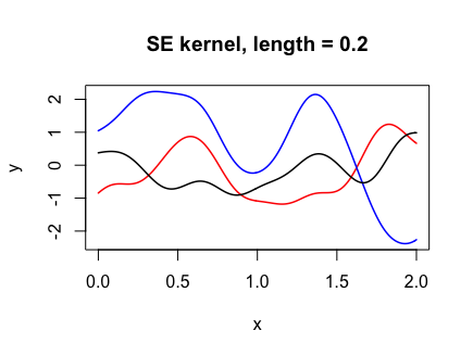
The following code shows how changing the “length-scale” parameter l affects the functions drawn. The smaller l is, the more wiggly the functions drawn.
par(mfrow = c(1, 3))
for (l in c(0.2, 0.7, 1.5)) {
    Y <- draw_samples(x, N, kernel_fn = se_kernel, length = l)

    plot(range(x), range(Y), xlab = "x", ylab = "y", type = "n",
         main = paste("SE kernel, length =", l))
    for (n in 1:N) {
        lines(x, Y[, n], col = col_list[n], lwd = 1.5)
    }
}

Rational quadratic (RQ) kernel
The rational quadratic (RQ) kernel has the form
 = \sigma^2 \left( 1 + \frac{\| x - x' \|^2}{2 \alpha l^2}\right)^{-\alpha}, \end{aligned}")
where 
rq_kernel <- function(x, y, alpha = 1, sigma = 1, length = 1) {
    sigma^2 * (1 + (x - y)^2 / (2 * alpha * length^2))^(-alpha)
}

par(mfrow = c(1, 3))
for (a in c(0.01, 0.5, 50)) {
    Y <- draw_samples(x, N, kernel_fn = rq_kernel, alpha = a)

    plot(range(x), range(Y), xlab = "x", ylab = "y", type = "n",
         main = paste("RQ kernel, alpha =", a))
    for (n in 1:N) {
        lines(x, Y[, n], col = col_list[n], lwd = 1.5)
    }
}

Matérn covariance functions
The Matérn covariance function has the form
 = \sigma^2 \frac{2^{1-\nu}}{\Gamma (\nu)} \left( \frac{\sqrt{2\nu} \|x-x'\|}{l}\right)^\nu K_\nu \left( \frac{\sqrt{2\nu} \|x-x'\|}{l} \right), \end{aligned}")
where 

matern_kernel <- function(x, y, nu = 1.5, sigma = 1, l = 1) {
    if (!(nu %in% c(0.5, 1.5, 2.5))) {
        stop("p must be equal to 0.5, 1.5 or 2.5")
    }
    p <- nu - 0.5
    d <- abs(x - y)
    if (p == 0) {
        sigma^2 * exp(- d / l)
    } else if (p == 1) {
        sigma^2 * (1 + sqrt(3)*d/l) * exp(- sqrt(3)*d/l)
    } else {
        sigma^2 * (1 + sqrt(5)*d/l + 5*d^2 / (3*l^2)) * exp(-sqrt(5)*d/l)
    }
}

par(mfrow = c(1, 3))
for (nu in c(0.5, 1.5, 2.5)) {
    Y <- draw_samples(x, N, kernel_fn = matern_kernel, nu = nu)

    plot(range(x), range(Y), xlab = "x", ylab = "y", type = "n",
         main = paste("Matern kernel, nu =", nu * 2, "/ 2"))
    for (n in 1:N) {
        lines(x, Y[, n], col = col_list[n], lwd = 1.5)
    }
}

The paths from the Matérn-1/2 kernel are often deemed too rough to be used in practice.
Periodic kernel
The periodic kernel has the form
![\begin{aligned} K(x, x') = \sigma^2 \exp \left[ - \frac{2 \sin^2 (\pi \| x - x'\| / p) }{l^2} \right], \end{aligned}](https://s0.wp.com/latex.php?latex=%5Cbegin%7Baligned%7D+K%28x%2C+x%27%29+%3D+%5Csigma%5E2+%5Cexp+%5Cleft%5B+-+%5Cfrac%7B2+%5Csin%5E2+%28%5Cpi+%5C%7C+x+-+x%27%5C%7C+%2F+p%29+%7D%7Bl%5E2%7D+%5Cright%5D%2C+%5Cend%7Baligned%7D&bg=ffffff&%23038;fg=333333&%23038;s=0 "\begin{aligned} K(x, x') = \sigma^2 \exp \left[ - \frac{2 \sin^2 (\pi \| x - x'\| / p) }{l^2} \right], \end{aligned}")
where
period_kernel <- function(x, y, p = 1, sigma = 1, length = 1) {
    sigma^2 * exp(-2 * sin(pi * abs(x - y) / p)^2 / length^2)
}

par(mfrow = c(1, 3))
for (p in c(0.5, 1, 2)) {
    Y <- draw_samples(x, N, kernel_fn = period_kernel, p = p)

    plot(range(x), range(Y), xlab = "x", ylab = "y", type = "n",
         main = paste("Periodic kernel, p =", p))
    for (n in 1:N) {
        lines(x, Y[, n], col = col_list[n], lwd = 1.5)
    }
}

Linear/polynomial kernel
The polynomial kernel has the form
 = (x^T x' + \sigma^2)^d, \end{aligned}")
where 

poly_kernel <- function(x, y, sigma = 1, d = 1) {
    (sigma^2 + x * y)^d
}

# linear kernel w different sigma
par(mfrow = c(1, 3))
for (s in c(0.5, 1, 5)) {
    Y <- draw_samples(x, N, kernel_fn = poly_kernel, sigma = s)

    plot(range(x), range(Y), xlab = "x", ylab = "y", type = "n",
         main = paste("Linear kernel, sigma =", s))
    for (n in 1:N) {
        lines(x, Y[, n], col = col_list[n], lwd = 1.5)
    }
}

# poly kernel of different dimensions
par(mfrow = c(1, 3))
for (d in c(1, 2, 3)) {
    Y <- draw_samples(x, N, kernel_fn = poly_kernel, d = d)

    plot(range(x), range(Y), xlab = "x", ylab = "y", type = "n",
         main = paste("Polynomial kernel, d =", d))
    for (n in 1:N) {
        lines(x, Y[, n], col = col_list[n], lwd = 1.5)
    }
}


Brownian motion
Brownian motion, the most studied object in stochastic processes, is a one-dimensional Gaussian process with mean zero and covariance function  = \min (x, x')")
bm_kernel <- function(x, y) {
    pmin(x, y)
}

Y <- draw_samples(x, N, kernel_fn = bm_kernel)

plot(range(x), range(Y), xlab = "x", ylab = "y", type = "n",
     main = "Brownian motion kernel")
for (n in 1:N) {
    lines(x, Y[, n], col = col_list[n], lwd = 1.5)
}
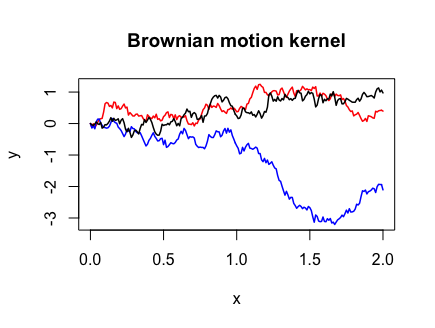
Note that I had to use the pmin() function instead of min() in the Brownian motion covariance function. This is because the outer(X, Y, FUN, ...) function we called in cov_matrix()
“…[extends
XandY] byrepto length the products of the lengths ofXandYbeforeFUNis called.” (fromouter()documentation)
pmin() would perform the operation we want, while min() would simply return the minimum value present in the two arguments, not what we want.
R-bloggers.com offers daily e-mail updates about R news and tutorials about learning R and many other topics. Click here if you're looking to post or find an R/data-science job.
Want to share your content on R-bloggers? click here if you have a blog, or here if you don't.