Working with spatial data is a key feature in ecological research. Using R to handle this type of data has the great advantage of keeping both variable extraction and modelling in the same environment, instead of recurring to external GIS softwares to compute some variables and then turning to R for modelling. In this example I’ll use as my base data an altimetry contour line map, then I’ll compute a DEM (digital elevation model) from the altimetry contour lines, derive some maps with variables related to altimetry and finally I’ll measure the variables for sampling sites.

In this example packages “rgdal” and “rgeos” are used to perform vectorial operations, package “raster” to obtain and work with raster maps package “gstat” to interpolation and packages “rgl” and “rasterVis” to visualize 3D plots.

library(raster)
library(rgdal)
library(rgeos)
library(gstat)
library(rgl)
library(rasterVis)

The base data can be downloaded here, and is composed of: 1) altimetry, 2) sampling points and 3) study area boundary. As the data is in vector format it can be imported with readOGR().

altimetry <- readOGR(dsn = ".", layer = "altimetry", verbose = F)
study_area <- readOGR(dsn = ".", layer = "study_area", verbose = F)
sampling_points <- readOGR(dsn = ".", layer = "sampling_points", verbose = F)

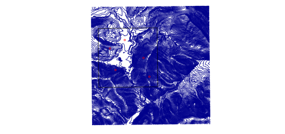
To visualize the data is best to plot all the different information in one plot.

# Plot contour lines
plot(altimetry, col = "dark blue")

# Add study area boundary
plot(study_area, add = TRUE)

# Add sampling points
points(sampling_points, col = "red", cex = 0.5)

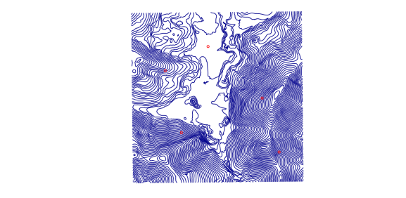
Spatial data manipulation can be very time consuming. So, it’s wise to clip the altimetry map to the study area to increase speed in further computations. Function intersection() can be used for this end. The new altimetry map is shown below.

# Clip altimetry map to study area
altimetry_clip <- intersect(altimetry, study_area)

# Plot clipped altimetry map
plot(altimetry_clip, col = "dark blue")

# Add sampling points
points(sampling_points, col = "red", cex = 0.5)

To create a DEM from altimetry contour lines the following steps are needed: 1) Create a blank raster grid to interpolate the elevation data onto; 2) Convert the contour lines to points so you can interpolate between elevation points; 3) Interpolate the elevation data onto the raster grid.

1. First we need to create a blank raster grid. The extent and the projection of the raster should be the same as the altimetry map, so we are going to use the information of this shape for our new raster grid. Afterwards the pixel size of the raster is also defined. In this example I’ll use a 5m x 5m pixel.

# Obtain extent
dem_bbox <- bbox(altimetry_clip)

# Create raster
dem_rast <- raster(xmn = dem_bbox[1, 1], 
                   xmx = ceiling(dem_bbox[1, 2]),
                   ymn = dem_bbox[2, 1], 
                   ymx = ceiling(dem_bbox[2, 2]))

# Set projection
projection(dem_rast) <- CRS(projection(altimetry_clip))

# Set resolution
res(dem_rast) <- 5

2. Since interpolation methods were conceived to work with point data, we need to convert the elevation contour lines to elevation points. Essentially we are creating points along each contour line that has as its value the elevation of the associated contour line.

# Convert to elevation points
dem_points <- as(altimetry_clip, "SpatialPointsDataFrame")

3. To perform the interpolation of the point data one two methods are widely used: Nearest Neighbor and Inverse Distance Weighted. The difference between the two methods is that in nearest neighbor all the surrounding points have the same weight. In inverse distance weighted points that are further away get less weight. The function used is the same, gstat(), but for the nearest neighbor methods the argument “idp”, the inverse distance power, must equal zero. For inverse distance some value of idp should be set.

# Compute the interpolation function
dem_interp <- gstat(formula = ALT ~ 1, locations = dem_points,
 set = list(idp = 0), nmax = 5)

# Obtain interpolation values for raster grid
DEM <- interpolate(dem_rast, dem_interp)

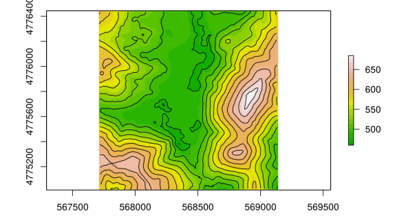
Now that we have our elevation model ready we can plot it in 2D with some contour lines added for better visualization.

# Subset contour lines to 20m to enhance visualization
contour_plot <- altimetry_clip[(altimetry_clip$ALT) %in% 
                                 seq(min(altimetry_clip$ALT), 
                                     max(altimetry_clip$ALT), 
                                     20), ]                                                                   
# Plot 2D DEM with contour lines
plot(DEM, col = terrain.colors(20))
plot(contour_plot, add = T)

Or make an interactive 3D plot that can be controlled with the mouse.

plot3D(DEM)

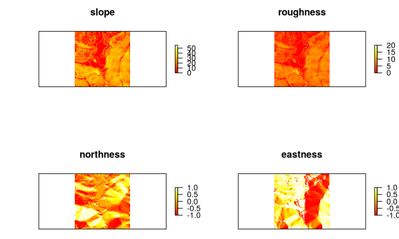
With the DEM ready other altitude related variables can be derived, such as slope, aspect or roughness, among others. As aspect is a circular variable, i. e., the minimum value (0º) and the maximum value (360º) represent the same thing (north), a better way of using this information is to convert it into two new variables: northness = cos(aspect) and eastness = sin(aspect). Please take note that aspect must be in radians (radian = degree * pi / 180). Northness will take values close to 1 if the aspect is mostly northward, close to -1 if the aspect is southward, and close to 0 if the aspect is either east or west. Eastness behaves similarly, except that values close to 1 represent east-facing slopes. Other approach would be to reclassify aspect into N, S, E and W.

# Obtain DEM derived maps
derived_vars <- terrain(DEM, opt = c('slope', 'roughness', 'aspect'), unit = "degrees")
slope <- derived_vars[["slope"]]
roughness <- derived_vars[["roughness"]]
northness <- cos(derived_vars[["aspect"]] * pi / 180)
eastness <- sin(derived_vars[["aspect"]] * pi / 180)

# Plot maps
par(mfrow = c(2, 2))
plot(slope, col = heat.colors(20), main = "slope", axes = F)
plot(roughness, col = heat.colors(20), main = "roughness", axes = F)
plot(northness, col = heat.colors(20), main = "northness", axes = F)
plot(eastness, col = heat.colors(20), main = "eastness", axes = F)

Having all the maps prepared, last thing to do is to measure the values of these maps in the sampling points and create a data frame that can be used in further modelling. A very simple way would be to just measure the values in the exact location of the points, but a better way is to use a buffer around the sampling points and summarize the values in the buffer, using mean, mode, max, etc.

# Create buffers with 100m radius around sampling points
sp_buff <- gBuffer(sampling_points, width = 100, 
                   quadsegs = 50, byid = TRUE)

# Measure variables in buffer area
sp_alt <- extract(DEM, sp_buff, fun = mean)
sp_slope <- extract(slope, sp_buff, fun = mean) 
sp_rough <- extract(roughness, sp_buff, fun = mean)
sp_north <- extract(northness, sp_buff, fun = mean)
sp_east <- extract(eastness, sp_buff, fun = mean)

# Prepare dataframe
results <- data.frame("id" = sp_buff@data$id,
                      "altitude" = sp_alt,
                      "slope" = sp_slope,
                      "roughness" = sp_rough,
                      "northness" = sp_north,
                      "eastness" = sp_east)
# View results
print(results)
##   id altitude     slope roughness   northness   eastness
## 1  1 487.2113  1.980742 0.4936204 -0.06990387  0.9496363
## 2  2 637.9079 26.458705 6.5107228  0.25682424 -0.9029607
## 3  3 534.3797 28.770571 7.0379747  0.93539489  0.2672350
## 4  4 537.3855 18.411266 4.4562798 -0.24734534  0.6485864
## 5  5 583.4479 27.955300 6.9689737 -0.28556347  0.8485821

Using R as GIS to handle spatial data not only the advantage of keeping both variable extraction and modelling in the same environment but also gives the possibility of creating a script to extract the variables, with the obvious advantages for future analysis.