
Quantitative Finance Applications in R – 6: Constructing a Term Structure of Interest Rates Using R (Part 1)
Want to share your content on R-bloggers? click here if you have a blog, or here if you don't.
by Daniel Hanson
Introduction
Last time, we used the discretization of a Brownian Motion process with a Monte Carlo method to simulate the returns of a single security, with the (rather strong) assumption of a fixed drift term and fixed volatility. We will return to this topic in a future article, as it relates to basic option pricing methods, which we will then expand upon.
For more advanced derivatives pricing methods, however, as well as an important topic in its own right, we will talk about implementing a term structure of interest rates using R. This will be broken up into two parts: 1) working with dates and interpolation (the subject of today’s article), and 2) calculating forward interest rates and discount factors (the topic of our next article), using the results presented below.
Working with Dates in R
The standard date objects in base R, to be honest, are not the most user-friendly when it comes to basic date calculations such as adding days, months, or years. For example, just to add, say, five years to a given date, we would need to do the following:
startDate <- as.Date('2014-05-27')
pDate <- as.POSIXlt(startDate)
endDate <- as.Date(paste(pDate$year + 1900 + 5, "-", pDate$mon + 1, "-", pDate$mday, sep = ""))
So, you’re probably asking yourself, “wouldn’t it be great if we could just add the years like this?”:
endDate <- startDate + years(5) # ?
Well, the good news is that we can, by using the lubridate package. In addition, instantiating a date is also easier, simply by indicating the date format (eg ymd(.) for year-mo-day) as the function. Below are some examples:
require(lubridate)
startDate <- ymd(20140527)
startDate # Result is: “2014-05-27 UTC”
anotherDate <- dmy(26102013)
anotherDate # Result is: “2013-10-26 UTC”
startDate + years(5) # Result is: “2019-05-27 UTC”
anotherDate – years(40) # Result is: “1973-10-26 UTC”
startDate + days(2) # Result is: “2014-05-29 UTC”
anotherDate – months(5) # Result is: “2013-05-26 UTC”
Remark: Note that “UTC” is appended to the end of each date, which indicates the Coordinated Universal Time time zone (the default). While it is not an issue in these examples, it will be important to specify a particular time zone when we set up our interpolated yield curve, as we shall see shortly.
Interpolation with Dates in R
When interpolating values in a time series in R, we revisit with our old friend, the xts package, which provides both linear and cubic spline interpolation. We will demonstrate this with a somewhat realistic example.
Suppose the market yield curve data on 2014-05-14 appears on a trader’s desk as follows:
Overnight ON 0.08%
One week 1W 0.125%
One month 1M 0.15%
Two months 2M 0.20%
Three months 3M 0.255%
Six months 6M 0.35%
Nine months 9M 0.55%
One year 1Y 1.65%
Two years 2Y 2.25%
Three years 3Y 2.85%
Five years 5Y 3.10%
Seven years 7Y 3.35%
Ten years 10Y 3.65%
Fifteen years 15Y 3.95%
Twenty years 20Y 4.65%
Twentyfive years 25Y 5.15%
Thirty years 30Y 5.85%
This is typical of yield curve data, where the dates get spread out farther over time. Each rate is a zero (coupon) rate, meaning that, in US Dollar parlance, the rate paid on $1 of debt today at a given point in the future, with no intermediate coupon payments; principal is returned and interest is paid in full at the end date. In order to have a fully functional term structure — that is, to be able to calculate forward interest rates and forward discount factors off of the yield curve for any two dates — we will need to interpolate the zero rates. The date from which the time periods are measured is often referred to as the “anchor date”, and we will adopt this terminology.
To start, we will use dates generated with lubridate operations to replicate the above yield curve data schedule. We will then match the dates up with the corresponding rates and put them into an xts object. We will use 2014-05-14 as our anchor date.
# ad = anchor date, tz = time zone
# (see http://en.wikipedia.org/wiki/List_of_tz_database_time_zones)
ad <- ymd(20140514, tz = "US/Pacific")
marketDates <- c(ad, ad + days(1), ad + weeks(1), ad + months(1), ad + months(2),
ad + months(3), ad + months(6), ad + months(9), ad + years(1), ad + years(2), ad + years(3), ad + years(5), ad + years(7), ad + years(10), ad + years(15),
ad + years(20), ad + years(25), ad + years(30))
# Use substring(.) to get rid of “UTC”/time zone after the dates
marketDates <- as.Date(substring(marketDates, 1, 10))
# Convert percentage formats to decimal by multiplying by 0.01:
marketRates <- c(0.0, 0.08, 0.125, 0.15, 0.20, 0.255, 0.35, 0.55, 1.65,
2.25, 2.85, 3.10, 3.35, 3.65, 3.95, 4.65, 5.15, 5.85) * 0.01
numRates <- length(marketRates)
marketData.xts <- as.xts(marketRates, order.by = marketDates)
head(marketData.xts)
# Gives us the result:
# [,1]
# 2014-05-14 0.00000
# 2014-05-15 0.00080
# 2014-05-21 0.00125
# 2014-06-14 0.00150
# 2014-07-14 0.00200
# 2014-08-14 0.00255
Note that in this example, we specified the time zone. This is important, as lubridate will automatically convert to your local time zone from UTC. If we hadn’t specified the time zone, then out here on the US west coast, depending on the time of day, we could get this result from the head(.) command; where the dates get converted to Pacific time; note how the dates end up shifted back one day:
[,1]
2014-05-13 0.00000
2014-05-14 0.00080
2014-05-20 0.00125
2014-06-13 0.00150
2014-07-13 0.00200
2014-08-13 0.00255
Some might call this a feature, and others may call it a quirk, but in any case, it is better to specify the time zone in order to get consistent results.
If we take a little trip back to our earlier post on plotting xts data (see section Using plot(.) in the xts package) a few months ago, we can have a look at a plot of our market data:
colnames(marketData.xts) <- "ZeroRate"
plot(x = marketData.xts[, “ZeroRate”], xlab = “Time”, ylab = “Zero Rate”,
main = “Market Zero Rates 2014-05-14”, ylim = c(0.0, 0.06),
major.ticks= “years”, minor.ticks = FALSE, col = “red”)
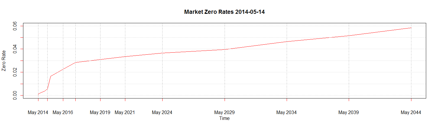
From here, the next steps will be:
- Create an empty xts object with daily dates spanning the anchor date out to 30 years
- Substitute in the known rates from the market yield curve
- Interpolate to fill in zero rates for the other dates
To create an empty xts object, we borrow an idea from the xts vignette, (Section 3.1, “Creating new data: the xts constructor”), and come up with the following function:
createEmptyTermStructureXtsLub <- function(anchorDate, plusYears)
{
# anchorDate is a lubridate here:
endDate <- anchorDate + years(plusYears)
numDays <- endDate - anchorDate
# We need to convert anchorDate to a standard R date to use
# the “+ 0:numDays” operation.
# Also, note that we need a total of numDays + 1 in order to capture both end points.
xts.termStruct <- xts(rep(NA, numDays + 1), as.Date(anchorDate) + 0:numDays)
return(xts.termStruct)
}
Then, using our anchor date ad (2014-05-14), we generate an empty xts object going out daily for 30 years:
termStruct <- createEmptyTermStructureXtsLub(ad, 30)
head(termStruct)
tail(termStruct)
# Results are (as desired):
# > head(termStruct)
# [,1]
# 2014-05-14 NA
# 2014-05-15 NA
# 2014-05-16 NA
# 2014-05-17 NA
# 2014-05-18 NA
# 2014-05-19 NA
# > tail(termStruct)
# [,1]
# 2044-05-09 NA
# 2044-05-10 NA
# 2044-05-11 NA
# 2044-05-12 NA
# 2044-05-13 NA
# 2044-05-14 NA
Next, substitute in the known rates from our market yield curve. While there is likely a slicker way to do this, a loop is transparent, easy to write, and doesn’t take all that long to execute in this case:
for(i in (1:numRates)) termStruct[marketDates[i]] <- marketData.xts[marketDates[i]]
head(termStruct, 8)
tail(termStruct)
# # Results are as follows. Note that we capture the market rates
# at ON, 1W, and 30Y:
# > head(termStruct, 8)
# [,1]
# 2014-05-14 0.00000
# 2014-05-15 0.00080
# 2014-05-16 NA
# 2014-05-17 NA
# 2014-05-18 NA
# 2014-05-19 NA
# 2014-05-20 NA
# 2014-05-21 0.00125
# > tail(termStruct)
# [,1]
# 2044-05-09 NA
# 2044-05-10 NA
# 2044-05-11 NA
# 2044-05-12 NA
# 2044-05-13 NA
# 2044-05-14 0.0585
Finally, we use interpolation methods provided in xts to fill in the rates in between. We have two choices, either linear interpolation, using the xts function na.approx(.), or cubic spline interpolation, using the function na.spline(.). As the names suggest, these functions will replace NA values in the xts object with interpolated values. Below, we show both options:
termStruct.lin.interpolate <- na.approx(termStruct)
termStruct.spline.interpolate <- na.spline(termStruct, method = "hyman")
head(termStruct.lin.interpolate, 8)
head(termStruct.spline.interpolate, 8)
tail(termStruct.lin.interpolate)
tail(termStruct.spline.interpolate)
# Results are as follows. Note again that we capture the market rates
# at ON, 1W, and 30Y:
# > head(termStruct.lin.interpolate, 8)
# ZeroRate
# 2014-05-14 0.000000
# 2014-05-15 0.000800
# 2014-05-16 0.000875
# 2014-05-18 0.001025
# 2014-05-19 0.001100
# 2014-05-20 0.001175
# 2014-05-21 0.001250
# > head(termStruct.spline.interpolate, 8)
# ZeroRate
# 2014-05-14 0.0000000000
# 2014-05-15 0.0008000000
# 2014-05-16 0.0009895833
# 2014-05-17 0.0011166667
# 2014-05-18 0.0011937500
# 2014-05-19 0.0012333333
# 2014-05-20 0.0012479167
# 2014-05-21 0.0012500000
# > tail(termStruct.lin.interpolate)
# ZeroRate
# 2044-05-09 0.05848084
# 2044-05-10 0.05848467
# 2044-05-11 0.05848851
# 2044-05-12 0.05849234
# 2044-05-13 0.05849617
# 2044-05-14 0.05850000
# > tail(termStruct.spline.interpolate)
# ZeroRate
# 2044-05-09 0.05847347
# 2044-05-10 0.05847877
# 2044-05-11 0.05848407
# 2044-05-12 0.05848938
# 2044-05-13 0.05849469
# 2044-05-14 0.05850000
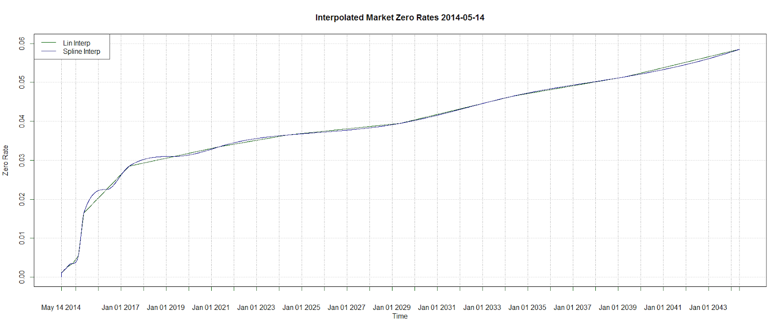
We can also have a look at the plots of the interpolated curves. Note that the linearly interpolated curve (in green) is the same as what we saw when we did a line plot of the market rates above:
plot(x = termStruct.lin.interpolate[, “ZeroRate”], xlab = “Time”, ylab = “Zero Rate”, main = “Interpolated Market Zero Rates 2014-05-14”,
ylim = c(0.0, 0.06), major.ticks= “years”, minor.ticks = FALSE,
col = “darkgreen”)
lines(x = termStruct.spline.interpolate[, “ZeroRate”],
col = “darkblue”)
legend(x = 'topleft', legend = c(“Lin Interp”, “Spline Interp”),
lty = 1, col = c(“darkgreen”, “darkblue”))
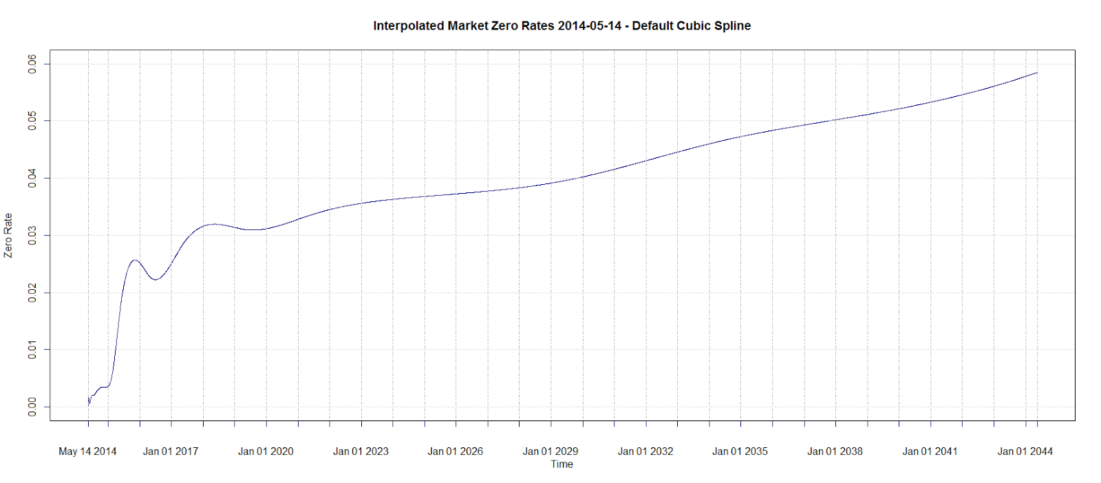
One final note: When we calculated the interpolated values using cubic splines earlier, we set method = “hyman” in the xts function na.spline(.). By doing this, we are able to preserve the monotonicity in the data points. Without it, using the default, we get dips in the curve between some of the data points, as shown here:
# Using the default method for cubic spline interpolation:
termStruct.spline.interpolate.default <- na.spline(termStruct)
colnames(termStruct.spline.interpolate.default) <- "ZeroRate"
plot(x = termStruct.spline.interpolate.default[, “ZeroRate”], xlab = “Time”,
ylab = “Zero Rate”,
main = “Interpolated Market Zero Rates 2014-05-14 –
Default Cubic Spline”,
ylim = c(0.0, 0.06), major.ticks= “years”,
minor.ticks = FALSE, col = “darkblue”)
Summary
In this article, we have demonstrated how one can take market zero rates, place them into an xts object, and then interpolate the rates in between the data points using the xts functions for linear and cubic spline interpolation. In an upcoming post — part 2 — we will discuss the essential term structure functions for calculating forward rates and forward discount factors.
For further and mathematically more detailed reading on the subject, the paper Smooth Interpolation of Zero Curves (Ken Adams, 2001) is highly recommended. A “financial cubic spline” as described in the paper would in fact be a useful option to have as a method in xts cubic spline interpolation.
R-bloggers.com offers daily e-mail updates about R news and tutorials about learning R and many other topics. Click here if you're looking to post or find an R/data-science job.
Want to share your content on R-bloggers? click here if you have a blog, or here if you don't.