
Probability distributions in R
Want to share your content on R-bloggers? click here if you have a blog, or here if you don't.
Some of the most fundamental functions in R, in my opinion, are those that deal with probability distributions. Whenever you compute a P-value you rely on a probability distribution, and there are many types out there. In this exercise I will cover four: Bernoulli, Binomial, Poisson, and Normal distributions. Let me begin with some theory first:
Bernoulli
Think of Bernoulli as a single coin flip, with probability of success 

} \right)")
with mean ")
Binomial
Think of Binomial as multiple independent Bernoulli trials, each with probabily of success 
")
with mean 
")

 = {n \choose x}p^x(1-p)^{n-x}")
so the probability of landing heads only once in 20 fair coin flips, for example, would be
 = {20 \choose 1}0.5^1(1-0.5)^{19} \approx 1.91 \times 10^{-5}")
turning out to be very, very unlikely.
Poisson
Think of Poisson as a the number of goals in a football match. Let 
")
with
Normal
Think of the Normal a.k.a. Gaussian distribution as the daily revenue from a local store. Let
")
with mean 

- The Central Limit Theorem (CLT) posits that no matter the shape of a particular distribution, the distribution of the sample mean (
) will follow a Normal distribution with
and
. This is key for distinguishing populations.
- The 68-95-99.7 rule posits that 68, 95 and 99.7% of the observations are contained in the intervals
,
and
, respectively.
- The standard Normal
is also a cornerstone in statistics. It simplifies many calculations since
. Variable standardization (Z-normalization) is nothing else but transforming a normally-distributed sample into a standard Normal using
, which explicitly mean-centers the data and scales for unit-variance (UV). This is often one of the first steps in predictive and inference modeling.
Let’s get started with R
We will now explore these distributions in R. Functions dealing with probability distributions in R have a single-letter prefix that defines the type of function we want to use. These prefixes are d, p, q and r. They refer to density/mass, cumulative, quantile and sampling functions, respectively. We will combine these prefixes with the names of the distributions we are interested in, which are binom (Bernoulli and Binomial), pois (Poisson) and norm (Normal). Note that a Binomial distribution with 
For starters, let us go back to the 20 coin flips example using 
")
n <- 1:20
den <- dbinom(n, 20, 0.7)
plot(den, ylab = "Density", xlab = "Number of successes")
sum(den) # = 1

The probability is maximum for 
Let us now turn to a different problem: the daily revenue of a local store follows a distribution ")


pnorm(1200,1000,200) # this gives us prob x smaller than 1200eur
1-pnorm(1200,1000,200) # this is the one, x greater than 1200eur
This probability is 
How about reversing the question? This is where quantiles become handy.
qnorm(1-0.16,1000,200) # = 1198.892
So not surprisingly, the 84th quantile is 
Finally, a demonstration of the CLT. Let us start with a Poisson distribution ")
n <- 1:20
den <- dpois(n, 3)
plot(den, xlab = "Outcome", ylab = "Density")
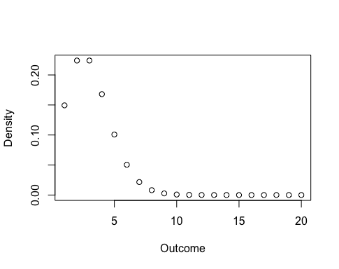
and we will draw 100 samples of 10 observations each. In each sample we will take the average value only. I will use set.seed to ensure you will draw the same random samples I did.
myMeans <- vector()
for(i in 1:100){
   set.seed(i)
   myMeans <- c(myMeans, mean(rpois(10,3)))
}
hist(myMeans, main = NULL, xlab = expression(bar(x)))

Looks not as normal as expected? That is because of the sample size. If you re-run the code above and replace 10 with 1000, you will obtain the following histogram.

Not only does the increased sample size improve the bell-shape, it also reduces the variance. Using the CLT we could successfully approximate 
Concluding,
- Model your data with the appropriate distribution according to the underlying assumptions. There is a tendency for disregarding simple distributions, when in fact they can help the most.
- While the definition of the Binomial and Poisson distributions is relatively straightforward, it is not so easy to ascertain ‘normality’ in a distribution of a continuous variable. A Box-Cox transformation might be helpful in resolving distributions skewed to different extents (and sign) into a Normal one.
- There are many other distributions out there – Exponential, Gamma, Beta, etc. The rule of the prefixes aforementioned for R still applies (e.g. pgamma, rbeta).
Enjoy!

R-bloggers.com offers daily e-mail updates about R news and tutorials about learning R and many other topics. Click here if you're looking to post or find an R/data-science job.
Want to share your content on R-bloggers? click here if you have a blog, or here if you don't.