Pilot Study: Small Town Land Surface Temperature
Want to share your content on R-bloggers? click here if you have a blog, or here if you don't.
Introduction
Zhang and Imhoff (2010) pdf here utilized NLCD impervious surface area (ISA), Olson biomes, and MODIS Land Surface temperature (LST) to estimate the magnitude of UHI in large cities across the US. Peng employed a similar approach in studying 419 large cities ( population greater than 1m ) around world. Peng’s work suggests a limit or threshold to the Surface Urban Heat Island (SUHI) effect in that he found that city size and population was not an effective predictor of SUHI for very large cities. Imhoff’s study on somewhat smaller cities suggest there is a range at which city size is an effective predictor of SUHI 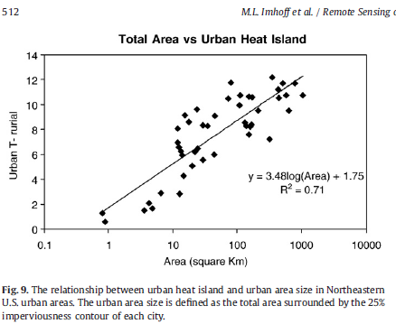
In addition, Zhang and Imhoff found that SUHI is related to the surrounding environment. A city that is developed in a forest biome, for example, will show a greater SHUI than one embedded in a desert.
Zhang and Imhoff’s curve is, as they note, somewhat similar to Oke’s postulated curve for the relationship between population and the Urban Heat Island ( UHI as measured by air temperature as opposed to surface temperature ) and it shares a certain weakness with Oke’s analysis with respect to the sample size at very small populations/small size. My goal in this study is to enlarge the sample of smaller sized cities and towns and refine the estimate in mch the same way that Peng focused his study on cities over 1M in population. My working hypothesis is that just as there is a plateau of SUHI above a certain size that there may be a plataeu at smaller sizes, suggesting that a logistic relationship might be a better representation of the underlying process.
Data
Data from a wide variety of sources was used to identify a set of candidate small cities and towns. The 2010 US census gazetter of places in the US was used to identify town and census designated places (CDP ) with land areas less than 10 sq km. NLCD 2006 ( ISA) 30 meter data and Nightlights derived ISA (1km data ) was used to narrow the list to small towns that are relatively isolated from larger urban areas. For the final processing Landcover provided by MODIS ( MOD12Q1 2005) (500 meter data ) was used to classify urban versus non urban pixels. As noted by Imhoff a cut off at 25% ISA by NLCD standard is consistent with Modis classification of urban pixels. A 1km Digital Elevation model derived from 90m SRTM data was utilized to compute elevations, slopes and aspects. Finally, 8 day 1km Day LST and Night LST from MODIS was used. For this pilot study one 8 day period from July 4th 2006 was utilized ( MOD11A2 v 5 )
Methods
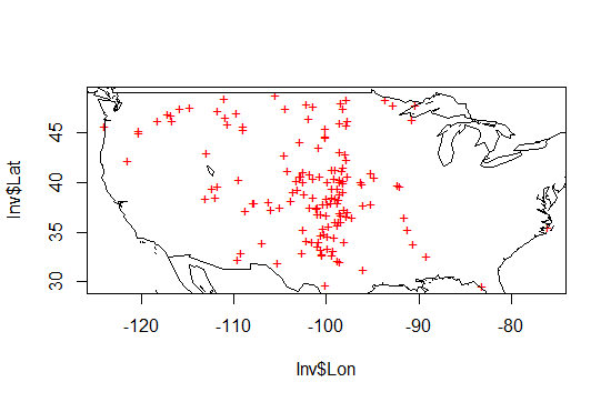
Census gazetter information was used to select a sample of small towns and CDPs that had areas less than 10 sq km and no substantial water area within the areas boundaries. That list was culled further using NLCD 2006 impervious area and Nightlights derived ISA to ensure that the small towns were at least 10km from larger urban areas. As Zhang/Imhoff Olson biomes were examined within .5 degrees of the site to ensure that the area existed in a singular biome and not an area that contained more than one biome. The final sample contained 169 sites spread out over the US as depicted below
 Individual datasets were then built for every site. MOD12Q1, MODIS landcover was collected for a ~60 km radius around each site. The landcover data was used to create several masks. An urban pixel mask, a rural pixel mask, and a water pixel mask. The urban pixel mask and the water pixel mask were used to create distance maps: Distance from urban pixel maps and distance from water maps. The elevation data was processed to create a slope map and aspect map for each 60km grid. Finally MODIS11A2 LST data was downloaded and reprojected to a geographic projection ( WGS84) at 1km resolution in GeoTiff format. Data “bricks” in Rs package “raster” were created for each site. Each brick consisted of a urban mask, rural mask, water mask, distance maps, terrain maps and temperature maps.
Some fun charts
The purpose of the pilot study was to assemble the data and start to build the analysis code base for a final production run. During that process some of my ideas and approaches to the problem have defininately changed. The first change was the decision to use MOD12Q1. The reason is clear. Looking at the processing chain for MOD11A2 ( LST ) it is clear that this data product relies on MOD12Q1 for its estimate of emmissivity. To put it simply if NLCD thinks the pixel is Urban or impervious and MOD12Q1 thinks the pixel is trees, then MOD11A2 will assume an emissivity of trees to calculate the final LST. The other thing that changed was my decision to include more terrain data than Zhang Imhoff. In their approach they masked off pixels that were 50meter higher or lower than the average in the urban area. In my approach I will look at using that terrain information to explain the variance we see. Finally, I will probably change my method of looking at the 50km radius around each site. In part this was done to make the calculations of distance maps less intense. I Will probably just go ahead and calculate distance maps for the whole US, a process that might take a couple days at 500meter resolution. That will allow me to sample a wider geographic variety of sites than I currently have which tends to be concentrated in the middle of the country and tends to over sample certain areas with many small isolated towns.
Now for some charts. First we see a sample chart from a given “brick” of data:
And next we see the Day LST and Night LST
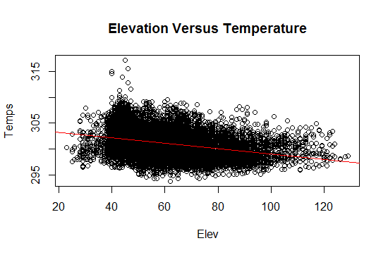
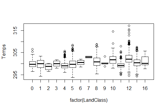
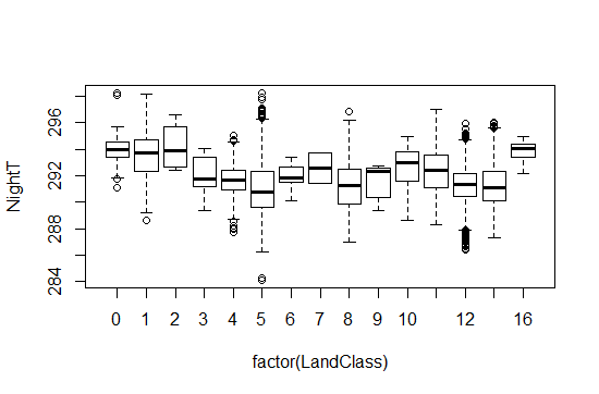
And for grins we look at the following: The ralationship between Temperature and Elevation for day and night, and below that we have box plots of the temperature versus the land cover types in the RURAL pixels. That is one other difference between Zhang/Imhoff and my work. Where they looked at the “biome” which is really a historical context I will look at the current land cover. The reason is simple: MODIS LST is dependendent opon MODIS landcover in its determination of emissivity and finally temperature.
Conclusion
You should note that I have not looked at the Urban rural difference yet. At this stage in the pilot study I don’t want to be looking at any of those results. I just want to get the processing chain bug free and the main routines ironed out. There will be a little more code to pull out the “area” of the small towns but that is pretty trivial. Next step now I think will be finding ways to speed up the calculation of the distance maps.
R-bloggers.com offers daily e-mail updates about R news and tutorials about learning R and many other topics. Click here if you're looking to post or find an R/data-science job.
Want to share your content on R-bloggers? click here if you have a blog, or here if you don't.


