Dataset:

state.x77 – Standard built-in dataset with 50 rows and 8 columns giving the following statistics in the respective columns.

Population: population estimate as of July 1, 1975

Income: per capita income (1974)

Illiteracy: illiteracy (1970, percent of population)

Life Exp: life expectancy in years (1969–71)

Murder: murder and non-negligent manslaughter rate per 100,000 population (1976)

HS Grad: percent high-school graduates (1970)

Frost: mean number of days with minimum temperature below freezing (1931–1960) in capital or large city

Area: land area in square miles

Response:

Conduct multiple regression to arrive at an optimal model which is able to predict the life expectancy .

We begin this exercise by running a few standard diagnostics on the data including by not limited to  head(), tail() , class(), str(), summary() ,names() etc.

The input dataset turns out to be a matrix which will need to be coerced into a data frame using as.data.frame().

Next,we’ll do a quick exploratory analysis on our data to examine the variables for outliers and distribution before proceeding. One way to do this is to plot qqplots for all the variables in the dataset.

for(i in 1:ncol(st)){
qqnorm(st[,i],main=colnames(st[,i]))
}

It’s a good idea to check the correlation between the variables to get a sense of the dependencies . We do this here using the cor(dataframe) function.

We can see that life expectancy appears to be moderately to strongly related to “Income” (positively), “Illiteracy” (negatively), “Murder” (negatively), “HS.Grad” (positively), and “Frost” (no. of days per year with frost, positively).

We can also view this by plotting our correlation matrix using pairs(dataframe)  which corroborates the cor.matrix  as seen above.

As a starting point for multiple regression would be to build a “full” model which will have Life Expectancy as the response variable and all other variables as explanatory variables. The summary of that linear model will be our “square one” and we will proceed to whittle it down until we reach our optimal model.

> model1 = lm(Life.Exp ~ ., data=st)
> summary(model1)

Call:
lm(formula = Life.Exp ~ ., data = st)

Residuals:
 Min         1Q     Median   3Q       Max 
-1.47514 -0.45887 -0.06352 0.59362 1.21823 

Coefficients:
             Estimate Std. Error t value Pr(>|t|) 
(Intercept) 6.995e+01  1.843e+00  37.956  < 2e-16 ***
Population  6.480e-05  3.001e-05   2.159   0.0367 * 
Income      2.701e-04  3.087e-04   0.875   0.3867 
Illiteracy  3.029e-01  4.024e-01   0.753   0.4559 
Murder     -3.286e-01  4.941e-02  -6.652   5.12e-08 ***
HS.Grad     4.291e-02  2.332e-02    1.840  0.0730 . 
Frost      -4.580e-03  3.189e-03   -1.436  0.1585 
Area       -1.558e-06  1.914e-06   -0.814  0.4205 
Density    -1.105e-03  7.312e-04   -1.511  0.1385 
---
Signif. codes: 0 ‘***’ 0.001 ‘**’ 0.01 ‘*’ 0.05 ‘.’ 0.1 ‘ ’ 1

Residual standard error: 0.7337 on 41 degrees of freedom
Multiple R-squared: 0.7501, Adjusted R-squared: 0.7013 
F-statistic: 15.38 on 8 and 41 DF, p-value: 3.787e-10

We see that this 70% of the variation in Life Expectancy is explained by all the variables together (Adjusted R-squared).

Let’s see if this can be made better. We’ll try to do that by removing one predictor at a time from model1, starting with “Illiteracy” (p-value = 0.4559 i.e. least significance) , until we have a model with all significant predictors.

> model2 = update(model1, .~. -Illiteracy)
> summary(model2)

Call:
lm(formula = Life.Exp ~ Population + Income + Murder + HS.Grad + 
 Frost + Area + Density, data = st)

Residuals:
 Min 1Q Median 3Q Max 
-1.47618 -0.38592 -0.05728 0.58817 1.42334 

Coefficients:
              Estimate Std. Error t value Pr(>|t|) 
(Intercept)  7.098e+01  1.228e+00   57.825   < 2e-16 ***
Population   5.675e-05  2.789e-05     2.034    0.0483 * 
Income       1.901e-04  2.883e-04     0.659    0.5133 
Murder       -3.122e-01 4.409e-02     -7.081    1.11e-08 ***
HS.Grad       3.652e-02 2.161e-02      1.690    0.0984 . 
Frost        -6.059e-03 2.499e-03      -2.425    0.0197 * 
Area         -8.638e-07 1.669e-06      -0.518     0.6075 
Density       -8.612e-04 6.523e-04       -1.320   0.1939 
---
Signif. codes: 0 ‘***’ 0.001 ‘**’ 0.01 ‘*’ 0.05 ‘.’ 0.1 ‘ ’ 1

Residual standard error: 0.7299 on 42 degrees of freedom
Multiple R-squared: 0.7466, Adjusted R-squared: 0.7044 
F-statistic: 17.68 on 7 and 42 DF, p-value: 1.12e-10

Next, Area must go (p-value = 0.6075!)

> model3 = update(model2, .~. -Area)
> summary(model3)

Call:
lm(formula = Life.Exp ~ Population + Income + Murder + HS.Grad + 
 Frost + Density, data = st)

Residuals:
 Min 1Q Median 3Q Max 
-1.49555 -0.41246 -0.05336 0.58399 1.50535 

Coefficients:
            Estimate Std. Error t value Pr(>|t|) 
(Intercept)  7.131e+01 1.042e+00 68.420 < 2e-16 ***
Population   5.811e-05 2.753e-05 2.110 0.0407 * 
Income       1.324e-04 2.636e-04 0.502 0.6181 
Murder      -3.208e-01 4.054e-02 -7.912 6.32e-10 ***
HS.Grad      3.499e-02 2.122e-02 1.649 0.1065 
Frost       -6.191e-03 2.465e-03 -2.512 0.0158 * 
Density     -7.324e-04 5.978e-04 -1.225 0.2272 
---
Signif. codes: 0 ‘***’ 0.001 ‘**’ 0.01 ‘*’ 0.05 ‘.’ 0.1 ‘ ’ 1

Residual standard error: 0.7236 on 43 degrees of freedom
Multiple R-squared: 0.745, Adjusted R-squared: 0.7094 
F-statistic: 20.94 on 6 and 43 DF, p-value: 2.632e-11

We will continue to throw out the predictors in this fashion . . . . .

> model4 = update(model3, .~. -Income)
> summary(model4)
> model5 = update(model4, .~. -Density)
> summary(model5)

. . . .  until we reach this point

> summary(model5)

Call:
lm(formula = Life.Exp ~ Population + Murder + HS.Grad + Frost, 
 data = st)

Residuals:
 Min 1Q Median 3Q Max 
-1.47095 -0.53464 -0.03701 0.57621 1.50683 

Coefficients:
              Estimate Std. Error t value Pr(>|t|) 
(Intercept)  7.103e+01 9.529e-01 74.542   < 2e-16 ***
Population   5.014e-05 2.512e-05 1.996     0.05201 . 
Murder      -3.001e-01 3.661e-02 -8.199    1.77e-10 ***
HS.Grad      4.658e-02 1.483e-02 3.142     0.00297 ** 
Frost       -5.943e-03 2.421e-03 -2.455    0.01802 * 
---
Signif. codes: 0 ‘***’ 0.001 ‘**’ 0.01 ‘*’ 0.05 ‘.’ 0.1 ‘ ’ 1

Residual standard error: 0.7197 on 45 degrees of freedom
Multiple R-squared: 0.736, Adjusted R-squared: 0.7126 
F-statistic: 31.37 on 4 and 45 DF, p-value: 1.696e-12

Now, here we have “Population” with a borderline p-value of 0.052 . Do we throw it out ? Do we keep it ? One way to know is to test for interactions.

> interact= lm(Life.Exp ~ Population * Murder * HS.Grad * Frost,data=st)
> anova(model5,interact)
Analysis of Variance Table

Model 1: Life.Exp ~ Population + Murder + HS.Grad + Frost
Model 2: Life.Exp ~ Population * Murder * HS.Grad * Frost
 Res.Df RSS Df Sum of Sq F Pr(>F) 
1 45 23.308 
2 34 14.235 11 9.0727 1.9699 0.06422 .
---
Signif. codes: 0 ‘***’ 0.001 ‘**’ 0.01 ‘*’ 0.05 ‘.’ 0.1 ‘ ’ 1

P-value of 0.06422 indicates that there is no significant interaction between the terms so we can drop “Population” as it doesn’t really contribute to anything at this point.BUT, if we drop “Population”, the adj R-squared drops a little as well . So as a trade-off, we’ll just keep it. 

So there you have it,folks.Our minimal optimal model with statistically significant slopes.

Run model diagnostics

par(mfrow=c(2,2)) # to view all 4 plots at once
plot(model5)

1. Residuals vs Fitted

We find equally spread residuals around a horizontal line without distinct patterns so that is a that is a good indication we don’t have non-linear relationships.

2. Normal Q-Q plot

#This plot shows if residuals are normally distributed. Our residuals more or less follow a straight line well, so that’s an encouraging sign.

3. Scale-location
This plot shows if residuals are spread equally along the ranges of predictors. This is how we can check the assumption of equal variance (homoscedasticity). It’s good that we can see a horizontal(-ish) line with equally (randomly) spread points.

4. Residuals vs Leverage

This plot helps us locate the influential cases that have an effect on the regression line.We look for subjects outside the dashed line , the Cook’s distance.The regression results will be altered if we exclude those cases.
‘Full’ model VS ‘Optimal’ model

> anova(model1,model5)
Analysis of Variance Table

Model 1: Life.Exp ~ Population + Income + Illiteracy + Murder + HS.Grad + 
 Frost + Area + Density
Model 2: Life.Exp ~ Population + Murder + HS.Grad + Frost
 Res.Df RSS Df Sum of Sq F Pr(>F)
1 41 22.068 
2 45 23.308 -4 -1.2397 0.5758 0.6818
>

The p-value of 0.6818 suggests that we haven’t lost any significance from when we started, so we’re good.

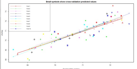
Onto some cross-validation

We will perform a 10-fold cross validation (m=10 in CVlm function).

A comparison of the cross- validation plots shows that model5 performs the best out of all other models.The lines of best fit are relatively parallel(-ish) and most big symbols are close to the lines indicating a decent accuracy of prediction.Also, the mean squared error is small , 0.6 .

cvResults <- suppressWarnings(CVlm(data=st, form.lm=model5, m=10, dots=FALSE, seed=29, legend.pos="topleft", printit=FALSE));

mean_squared_error <- attr(cvResults, 'ms')

The relative importance of predictors

The relaimpo package provides measures of relative importance for each of the predictors in the model.

install.packages("relaimpo")
library(relaimpo)
 

 calc.relimp(model5,type=c("lmg","last","first","pratt"),
 rela=TRUE)
 
 # Bootstrap Measures of Relative Importance (1000 samples) 
 boot <- boot.relimp(model5, b = 1000, type = c("lmg", 
 "last", "first", "pratt"), rank = TRUE, 
 diff = TRUE, rela = TRUE)
 booteval.relimp(boot) 

# print result
 plot(booteval.relimp(boot,sort=TRUE)) # plot result

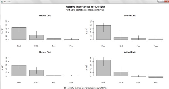
Yup. ‘Murder’ is the most important predictor of Life Expectancy, followed by ‘HS.Grad’ and ‘Frost. ‘Population’  sits smug at the other end of the spectrum with marginal effect and importance.

Well, looks like this is as good as it is going to get with this model.

I will leave you here, folks. Please feel free to work through various datasets (as I will) to get a firm grasp on things.

Did you find this article helpful?  Can it be improved upon ? Please leave me a comment !

Until next time!