
Learning gganimate with the LastFM API
Want to share your content on R-bloggers? click here if you have a blog, or here if you don't.
I’m one of the few people that actually still has – and uses – a Last.fm account. I say still, I’m one of the few who ever had one. I’ve been playing around with some APIs for the first time lately and thought I’d check out the Last.fm one. I decided my listening history was the perfect data to learn how to create a bar chart race. The code for this post can be found on my github page.
Getting started with the API.
I used the R package called scrobbler to get my data. Just sign in to last.fm, go to their dev site, and request an API key. Store your details as variables and plug them into the download_scrobbles() function from scrobbler. This will download your listening history as a dataframe.
username <- "YourUsername"
apiKey <- "YourAPIkey"
apiSecret <- "YourAPIsecret"

lastFM <- download_scrobbles(username = username, api_key = apiKey)
Mine had 89 pages of data – about 88,500 songs over 10 years. This took a long time to download so I recommend saving this dataframe so you don’t need to do this step again if you clear your environment at any point.
# Save file to prevent redownloading later
write.csv(lastFM, file = "lastFMfromAPI.csv")
Now that the data is downloaded, I’m going to subset it to only the variables I care about – the song title, artist, album, and date it was played.
# subset to only relevant data - song, artist, album, date
lastFM2 <- lastFM[,c(1,4,6,8)]
Data cleanup
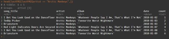
Let’s take a look at our data as it is now using the head() function.

In order to create our racing bar chart, we’ll need to group our data by month. So we’ll need to create a variable in our dataframe containing the month. Let’s tidy up our date column to make this easier. As with any time/date problem in R, we’ll use the lubridate package. First things first, let’s take the timestamp out of our date column.
# remove time from output
lastFM2$date <- gsub(",.*","",lastFM2$date)    # regex - removes everything after a comma (inclusive of comma)
Now we’ll use lubridate to convert the data type of the column to a date.
lastFM2$date <- lubridate::dmy(lastFM2$date) #dmy as date is ordered Day/Month/year
One of the issues with the dataset is a lot of the entries don’t have the right date associated with them. Anything that was scrobbled (last.fm’s word for recording when a track is played) on iTunes before I made the switch to Spotify has the timestamp 01-01-1970. Here I generated a random date to go with these entries. I chose the range of 01/01/2010 – 06/04/2011 (the earliest real date in the dataset). I’ll use the runif() function to generate these dates.
# Sort by date
lastFM2 <- lastFM2[order(lastFM2$date),]

head(unique(lastFM2$date)) # to get earliest real date

# Set these to a random date in the window 2010/01/01 - 2011/04/06 (ymd format)
# 14610 is UNIX date for 2010/01/01
# 15070 is UNIX date for 2011/04/06 (earliest track with accurate timestamp)
as_date(floor(runif(n = 1, min = 14610, max = 15070)))                         # test to get date
In the above runif() function, I’ve used n = 1 to give just one output. In order to replace the dates in our dataframe, I’ll need to know how many 1970s we have.
# Count number of entries with 1970 as date
count1970 <- length(lastFM2[lastFM2$date <= "1971-01-01",4])
And now replace the dates for the 1970s entries with random dates.
lastFM2[lastFM2$date <= "1971-01-01",4]<- as_date(floor(runif(n = count1970, min = 14610, max = 15070)))
Once again I’ll sort the data by date. I’ll want to get a running total for how many plays each artist has so it’s important to ensure our data is still in the right order.
# Order from oldest to newest
lastFM2 <- lastFM2[order(lastFM2$date),]
In order to get the running total, I’ll use the group_by() and mutate() functions from the dplyr package.
# 3.2 adds running total number of plays for each artist
lastFM2 <- lastFM2 %>% group_by(artist) %>%
  mutate(count=row_number())
Now we have one more column in our dataframe. Count keeps the running total for the number of plays an artist has. If we use the head() function to call a specific artist, we’ll see their songs in order of when they were listened to, and the count increasing by one for each play.
Now, let’s split our date up into year and month. Having one column for each will be helpful later on.
# 3.3 split date into year and month columns
lastFM2$year <- year(lastFM2$date)
lastFM2$month <- month(lastFM2$date)
One of the reasons we’re splitting our date up is to create a new column we’ll call monthID. This is just to differentiate the same month in different years. As things are, January 2010 and January 2011 are both down as month number 1. monthID will increment over time so January 2010 has ID 1, January 2011 has ID 13, etc. We’ll use this column to power our animation later.
# Add monthID column so same month in different years has different chronology
# Jan 2010 is month 1, Feb 2010 is month 2
# Jan 2011 should be month 13, Feb 2011 month 14 etc.
lastFM2$monthID <- lastFM2$month + ((lastFM2$year - 2010)*12)
Now I’ll remove the day from our date variable and group all of the entries by artist, monthID, and date. Again, we need to sort chronologically, so we’ll sort this new dataframe by monthID,
# Change date to remove day var
lastFM2$date <- format(lastFM2$date, format="%m-%y")

# Grouped by month
lastFMGrouped <- group_by(lastFM2, artist, monthID, date) %>%
  summarise(count = max(count))

# 3.7 Order grouped df chronologically
lastFMGrouped <- lastFMGrouped[order(lastFMGrouped$monthID),]

However, there is an issue here. One that I didn’t find until I created an animation and bars were jumping all over the place. Here is a snapshot of the total play count for the Red Hot Chili Peppers over a few months. RHCP did not receive any plays in August 2012, monthID 32. Ideally the count variable for month 32 for Red Hot Chili Peppers would read 2560, the same as the previous month they were present. This meant in our animation they were present (top, even) in month 31, absent in month 32, and top again in month 33. This isn’t what we want. My solution for this is pretty inelegant, and required me to take the data into Excel as I couldn’t work it out in R. If you can suggest a way to do this in R please let me know.
I started by taking a list of every artist, every date, and every monthID in the data and combined them in a new dataframe. I wanted an entry for every artist, every month. My data contained 3,425 different artists and 124 months, so this new dataframe was 424,700 rows long (3,425*124).
# Get every artist name and all dates/monthIDs
allBands <- unique(lastFMGrouped$artist)
allMonthIDs <- unique(lastFMGrouped$monthID)
allDates <- unique(lastFMGrouped$date)

# Create new df with all artists gaving 0 plays every month
newDF <- data.frame(artist = rep(allBands, 124),            # add every artist (length(allDates)) times
                    monthID = rep(allMonthIDs, 3425),       # add every monthID (length(allBands)) times
                    date = rep(allDates, 3425),             # add every date (length(allBands)) times
                    count = rep(0,424700))                  # set count = 0 for all of these
I used dplyr’s full_join() function to combine newDF and lastFMGrouped. I grouped the data as above once more and saved it to take into Excel.
# 4.3 combine this with grouped dataset
allArtistsAllDates <- full_join(lastFMGrouped, newDF)

# 4.4 group by artist and month/date again
allArtistsAllDates <- group_by(allArtistsAllDates, artist, monthID, date, .drop = F) %>%
  summarise(count = max(count))

# 4.5 save to take into excel
write.csv(allArtistsAllDates, file = "allArtistsAllDates.csv")
Excel data cleaning

Once I had the data in Excel, preparing it didn’t take too long. I added a column entitled maxcount to hold the highest the count has reached for that artist. The formula used in cell F3 is below.
=IF(B3=B2, IF(E3=E2, F2,MAX(E2:E3)),0)
Let’s break it down step by step:
=IF(B3=B2,         # Only if the artist doesn't change
IF(E3=E2,          # Check if the count variable changed from the previous row
F2,                # If it hasn't changed, the max is the same as it was before
MAX(E2:E3)         # If it has changed, set it to the higher value
),0)               # If the artist has changed, reset this value to 0
One more important note – Notice in the screenshot above the dates show the first six days of October. Our date was formatted mm/yy. Our first six entries (January-June 2010) are 01/10-06/10. When excel sees a date as this it assumes the format is dd/mm. We can fix this easily, just insert the below formula in cell G2 and double click the fill handle to copy it in every row.
=DATE(2010, C2, 1)
The =DATE formula formats a date in YMD, and here we are telling Excel to print a date that is the first day of the nth month of 2010, where n is our monthID. You can then select this column and paste it (as values) over the date column to put it back as it was. Make sure to delete the column from excel or your dataframe when you take it back into R will have an empty column.
Removing unnecessary values in Excel
I want to make this new file a bit smaller. As it is, we have 424,701 rows, but we don’t need that many. I wanted to insert the max value an artist had so far, so they need a row in every month after their first play. For example, I didn’t listen to *NSYNC until month 80 – I don’t need to keep the first 79 rows of *NSYNC that all have count zero. I only need the rows where count has a value >=1. This can be done easily enough in R, but since I have Excel open I’ll do it here. Apply a filter to your data to show only rows that have a maxcount of 0. Select all of these rows, right click and select “Delete Row”. That’s it – these data are gone. We’ve gone from 424,000 rows to 155,000. More detail on how to do this can be found here. Turn your filter off, convert your formulae to values and save as csv to bring back into R.
Back to R
Almost there, now it’s time to put our data into the right format for gganimate. Read in the csv file you’ve just saved in Excel and we’ll create a table with our top ten most played artists each month. note – this is not the month’s top artists, but our all-time top ten at that point in time.
# load in new csv manually created above/edited in excel
lastFMGrouped2 <- read.csv(file = "cleanedGrouped.csv", stringsAsFactors = F)

# Create table for use in plot
# Takes the top 10 most all time played artists each month - adds ranking column
lastFmTable <- lastFMGrouped2 %>%
  group_by(monthID) %>%
  mutate(rank = min_rank(-maxcount) *1) %>%       # multiply by one so type is numeric - not integer. Allows gganimate to place it in between integer places when moving
  filter(rank <= 10) %>%
  ungroup()
Each artist is also given a rank in this step, their place in the top 10 this month. This will be our x-variable in our plot. Once again, we need to reorder our dataframe by monthID, but don’t worry – this is the last time.
# Reorder by month
lastFmTable <- lastFmTable[order(lastFmTable$monthID),]
At this point you might need to tweak your data a bit. I manually removed a couple of ties and subset the data to start the animation a couple of years into the data. The first two years (the randomly generated data) moved so much and so quickly it wasn’t a pleasant viewing experience. I also used gsub() to add a line break to band names like “Red Hot Chili Peppers” that were wider than the bars on the chart. I also added one more column entitled ordering, which was just the inverse of the rank variable – where rank = 10, ordering = 1; where rank = 9, ordering = 2, etc. See the full code on github for more info on how that was done.
Below is all the code for the ggplot and for the animation.
# 7. ggplot  + gganimate
plot <- lastFmTable %>%

  ggplot(aes(ordering,
             group = artist)) +

  geom_tile(aes(y = maxcount/2,
                height = maxcount,
                width = 0.9,
                fill = artist),
            alpha = 0.9,
            colour = "Black",
            size = 0.75) +

  # text on top of bars
  geom_text(aes(y = maxcount, label = artist),
            vjust = -0.5) +

  # text in x-axis (requires clip = "off" in coord_cartesian)
  geom_text(aes(y = 0,
                label = artist),
            vjust = 1.1) +

  # label showing the month/year in the top left corner
  geom_label(aes(x=1.5,
                 y=4300,
                 label=paste0(date)),
             size=8,
             color = 'black') +

  coord_cartesian(clip = "off",
                  expand = FALSE) +

  labs(title = 'My most played artist over time.',
       subtitle = "My top lastFM artists from January 2011 to April 2020.",
       caption = '\n \n\nsource: lastFM | plot by @statnamara',
       x = '',
       y = '') +


  theme(
    plot.title = element_text(size = 18),
    axis.ticks.x = element_blank(),
    axis.text.x  = element_blank(),
    legend.position = "none",
  ) +

  transition_states(monthID,
                    transition_length = 20,
                    state_length = 2,
                    wrap = F) +             # wrap = F prevents the last frame being an in-between of the last and first months

  ease_aes('cubic-in-out')


animate(plot,
        duration = 48,           # seconds
        fps = 20,
        detail = 20,
        width = 1000,           # px
        height = 700,           # px
        end_pause = 90)         # number of frames to freeze on the last frame

anim_save(filename = "lastFM.gif", animation = last_animation())
The code above produces the animation seen here.

So that’s how I created my first gganimation. I have to recommend two great blog posts, here and here, that helped me greatly with this, as well as these two brilliant posts on stackoverflow on improving the animation. Post 1 / Post 2. And obviously I feel I should thank The Darkness, for clearly being the soundtrack to my life for the last 2-3 years. I couldn’t have done it without you.
R-bloggers.com offers daily e-mail updates about R news and tutorials about learning R and many other topics. Click here if you're looking to post or find an R/data-science job.
Want to share your content on R-bloggers? click here if you have a blog, or here if you don't.