
Generalized Additive Models
Want to share your content on R-bloggers? click here if you have a blog, or here if you don't.
This is also a flexible and smooth technique which captures the Non linearities in the data and helps us to fit Non linear Models.In this article I am going to discuss the implementation of GAMs in R using the 'gam' package .Simply saying GAMs are just a Generalized version of Linear Models in which the Predictors \(X_i\) depend Linearly or Non linearly on some Smooth Non Linear functions like Splines , Polynomials or Step functions etc.
The Regression Function \(F(x) \) gets modified in Generalized Additive Models , and only due to this transformation the GAMs are better in terms of Generalization to random unseen data , fits the data very smoothly and flexibly without adding Complexities or much variance to the Model most of the times.
The basic idea in Splines is that we are going to fit Smooth Non linear Functions on a bunch of Predictors \(X_i\) . Additive in the name means we are going to fit and retain the additivity of the Linear Models.
The Regression Equation becomes:
$$f(x) \ = y_i \ = \alpha \ + f_1(x_{i1}) \ + f_2(x_{i2}) \ + …. f_p(x_{ip}) \ + \epsilon_i$$
where the functions \(f_1,f_2,f_3,….f_p \) are different Non Linear Functions on variables \(X_p\) .
Let’s begin with its Implementation in R —
We will use the gam() function in R to fit a GAM.
#requiring the Package
require(gam)

#ISLR package contains the 'Wage' Dataset
require(ISLR)
attach(Wage) #Mid-Atlantic Wage Data

?Wage # To search more on the dataset
?gam() # To search on the gam function

gam1<-gam(wage~s(age,df=6)+s(year,df=6)+education ,data = Wage)
#in the above function s() is the shorthand for fitting smoothing splines
#in gam() function

summary(gam1)
##
## Call: gam(formula = wage ~ s(age, df = 6) + s(year, df = 6) + education,
##     data = Wage)
## Deviance Residuals:
##     Min      1Q  Median      3Q     Max
## -119.89  -19.73   -3.28   14.27  214.45
##
## (Dispersion Parameter for gaussian family taken to be 1235.516)
##
##     Null Deviance: 5222086 on 2999 degrees of freedom
## Residual Deviance: 3685543 on 2983 degrees of freedom
## AIC: 29890.31
##
## Number of Local Scoring Iterations: 2
##
## Anova for Parametric Effects
##                   Df  Sum Sq Mean Sq F value    Pr(>F)
## s(age, df = 6)     1  200717  200717 162.456 < 2.2e-16 ***
## s(year, df = 6)    1   22090   22090  17.879 2.425e-05 ***
## education          4 1069323  267331 216.372 < 2.2e-16 ***
## Residuals       2983 3685543    1236
## ---
## Signif. codes:  0 '***' 0.001 '**' 0.01 '*' 0.05 '.' 0.1 ' ' 1
##
## Anova for Nonparametric Effects
##                 Npar Df  Npar F  Pr(F)
## (Intercept)
## s(age, df = 6)        5 26.2089 <2e-16 ***
## s(year, df = 6)       5  1.0144 0.4074
## education
## ---
## Signif. codes:  0 '***' 0.001 '**' 0.01 '*' 0.05 '.' 0.1 ' ' 1
Now in the above code we are fitting a GAM which is Non linear in ‘age’ and ‘year’ with 6 degrees of freedom because they are fitted using Smoothing Splines , whereas it is Linear in Terms of variable ‘education’.
Plotting the Model
#Plotting the Model
par(mfrow=c(1,3)) #to partition the Plotting Window
plot(gam1,se = TRUE)
#se stands for standard error Bands
Gives this plot:

The above image has 3 different plots for each variable included in the Model.The X-axis contains the variable values itself and the Y-axis contains the Response values i.e the Salaries.
From the plots and their shapes we can see that Salary first increases with ‘age’ then decreases after around 60.For variable ‘year’ the Salaries tend to increase , and it seems that there is a decrease in salary at around year 2007 or 2008. And for the Categorical variable ‘education’ , Salary also increases monotonically. The curvy shapes for the variables ‘age’ and ‘year’ is due to the Smoothing splines which models the Non linearities in the data.The dotted Lines around the main curve lines are the Standard Error Bands.
Hence this is a very effective way of fitting Non linear functions on several variables and producing the plots for each and study the effect on the Response.
Logistic Regression using GAM
We can also fit a Logistic Regression Model using GAMs for predicting the Probabilities of the Binary Response values. We will use the identity I() function to convert the Response to a Binary variable.
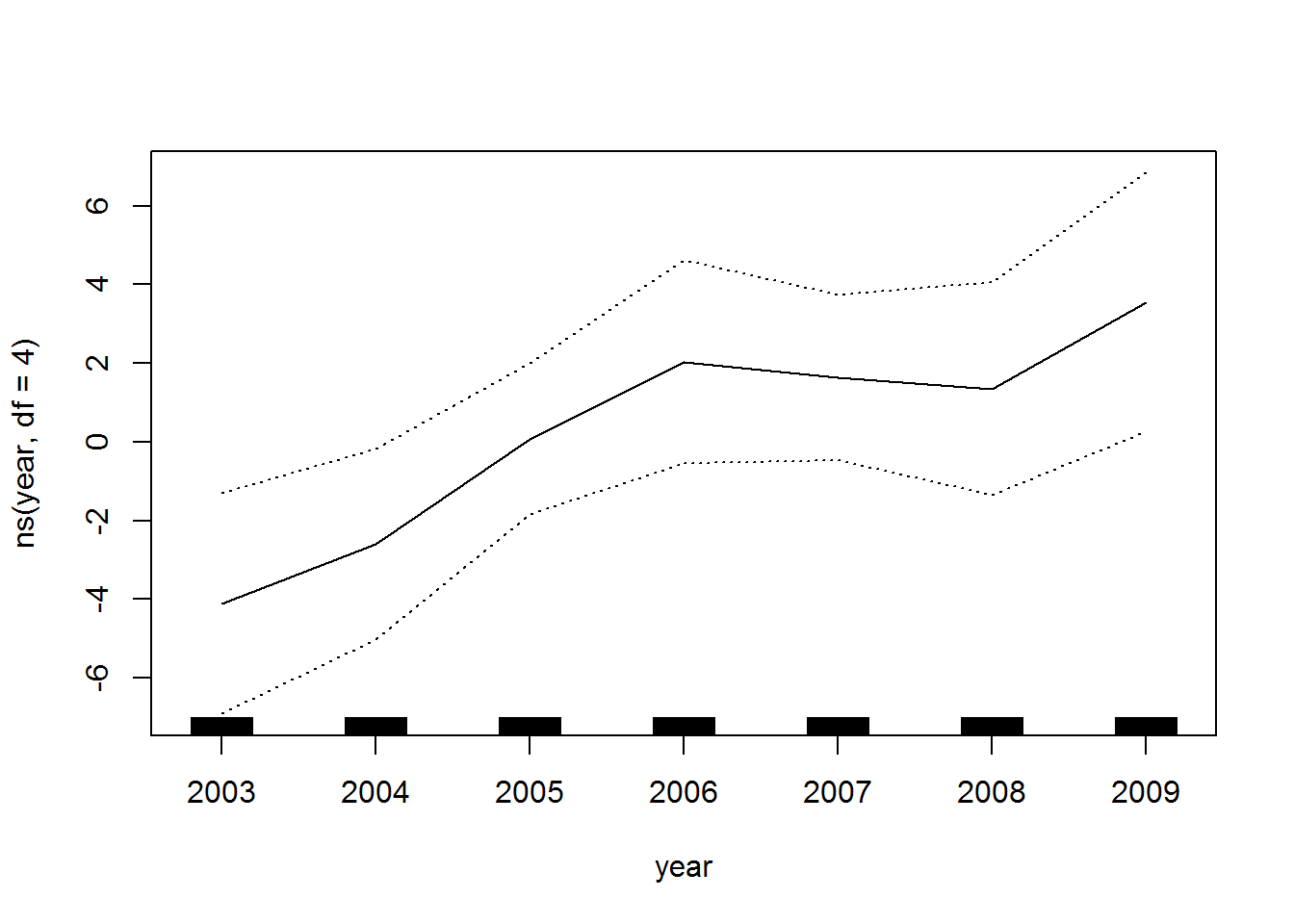
#logistic Regression Model
logitgam1<-gam(I(wage > 250) ~ s(age,df=4) + s(year,df=4) + education ,data=Wage,family=binomial)
plot(logitgam1,se=T)
In this Logistic Regression Model we are trying to find the conditional probability for the Wage variable which can take 2 values either, \( P(wage>250 \ | \ X_i) \) and \( P(wage<250 \ | \ X_i) \).
Gives this plot:


The above Plots are the same as the first Model,difference is that the Y-axis will now be the Logit \( log\frac{P(X)}{(1-P(X))} \) of the Probability values , and we now fit using 4 degrees of freedom for the variables ‘age’ and ‘year’ and again linear in terms of ‘education’ variable.
In the above Plot for ‘Year’ variable we can see that the error bands are quiet wide and broad.This might be an indication that our Non linear function fitted for ‘Year’ variable is not significant.
Now we can also check if we need Non linear terms for Year using Anova Test
We are now going to fit another model which in Linear in variable ‘year’.
#fitting the Additive Regression Model which is linear in Year
logitgam2<-gam(I(wage >250) ~ s(age,df=4)+ year + education , data =Wage, family = binomial)
plot(logitgam2)
Gives this plot:


Now for this Model,we don’t fit a Non linear function on ‘year’ variable , and it is simply a linear function in nature.As we can analyze from the plot above for ‘year’ , it is linear i.e a straight line (a polynomial of degree 1).
Now we will use anova() function in R for checking the goodness of fit for the above models, one which is Non Linear in Year and another which is Linear in Year.
#anova() function to test the goodness of fit and choose the best Model
#Using Chi-squared Non parametric Test due to Binary Classification Problem and categorical Target

anova(logitgam1,logitgam2,test = "Chisq")
## Analysis of Deviance Table
##
## Model 1: I(wage > 250) ~ s(age, df = 4) + s(year, df = 4) + education
## Model 2: I(wage > 250) ~ s(age, df = 4) + year + education
##   Resid. Df Resid. Dev Df Deviance Pr(>Chi)
## 1      2987     602.87
## 2      2990     603.78 -3 -0.90498   0.8242
The above results indicate that Model 2 i.e the one which is linear in terms of ‘year’ variable is significant and much better.Hence this indicates that we don’t need a GAM which fits a Non linear function for variable ‘year’.
Another way of Fitting a GAM
Now we can also fit a Generalized Additive Model using the lm() function in R,which stands for linear Model.And then we can fit Non linear functions on different variables \(X_i\) using the ns() or bs() function which stands for natural splines and cubic splines and add them to the Regression Model.
lm1<-lm(wage ~ ns(age,df=4) + ns(year,df=4)+ education , data  = Wage)
#ns() is function used to fit a Natural Cubic Spline
lm1

#Now plotting the Model

plot.gam(lm1,se=T)
##
## Call:
## lm(formula = wage ~ ns(age, df = 4) + ns(year, df = 4) + education,
##     data = Wage)
##
## Coefficients:
##                 (Intercept)             ns(age, df = 4)1
##                      43.976                       46.541
##            ns(age, df = 4)2             ns(age, df = 4)3
##                      29.070                       63.853
##            ns(age, df = 4)4            ns(year, df = 4)1
##                      10.881                        8.417
##           ns(year, df = 4)2            ns(year, df = 4)3
##                       3.596                        8.000
##           ns(year, df = 4)4          education2. HS Grad
##                       6.701                       10.870
##    education3. Some College     education4. College Grad
##                      23.354                       38.112
## education5. Advanced Degree
##                      62.517
Gives this plot:


Hence as the plot shows that the output of lm() function is also similar and same.It does not makes a difference if we use gam() or lm() to fit Generalized Additive Models.Both produce exactly same results.
Conclusion
Generalized Additive Models are a very nice and effective way of fitting Non linear Models which are smooth and flexible.Best part is that they lead to interpretable Models. We can easily mix terms in GAMs,some linear and some Non Linear terms and then compare those Models using the anova() function which performs a Anova test for goodness of fit.The non linear terms on Predictors \(X_i\) can be anything from smoothing splines , natural cubic splines to polynomial functions or step functions etc. GAMs are additive in nature , which means there are no interaction terms in the Model.
Thanks a lot for reading the article,and make sure to like and share it.Cheers!
Related Post
- Second step with non-linear regression: adding predictors
- Weather forecast with regression models – part 4
- Weather forecast with regression models – part 3
- Weather forecast with regression models – part 2
- Weather forecast with regression models – part 1
R-bloggers.com offers daily e-mail updates about R news and tutorials about learning R and many other topics. Click here if you're looking to post or find an R/data-science job.
Want to share your content on R-bloggers? click here if you have a blog, or here if you don't.