I can’t quite remember when I came up with the idea for this one, but I have a feeling this was a 3AM idea. I know the title doesn’t tell you much. I’m not talking about a Kramer Vs. Kramer reboot. Stone Cold Steve Austin isn’t coming out of retirement to fight YouTuber Austin McConnell. No, here I intend to answer an age old question. Are there more people with the name Austin in the United States, or are there more people in the city of Austin, Texas?

Now obviously, cities are big. Especially in America (at least to my Irish eyes). So the answer seems to be obviously the cities dumb-dumb. And not to mention that question can probably be answered with two google searches. So I did what anyone would do. I found as many American cities with people names as I could.

Using this Wikipedia page I skimmed the list and made a note of any cities that were applicable. For the names, I found US census data on Kaggle. With our data chosen, let’s get coding.

Austin-tatious data preparation

For the first pass at this, I decided to take just the ten most populous cities. Don’t worry, we’ll check more later

The first thing we’ll do is to create a variable with the names we want to check stored inside. We can also import our names dataset we downloaded from Kaggle and take a look at the first six rows using the head() function.

# Make a vector containing the names of the cities we want to check against.
cities <- c("Austin","Charlotte","Antonio","Diego","Jose","Jackson","Louis","Ana","Paul","Wayne")

# Import name dataset
nameData <- read.csv("NationalNames.csv")
head(nameData)

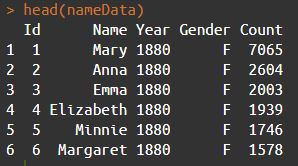
Using the head() function gives us the quick overview we need to see what kind of trimming we need to do. We can see that in the year 1880, there were 7,065 Marys born in the States. I donn’t want to check if every Austin ever outweighs the current population of the city – I just want to know if there are more living Austins. Google tells me that the US life expectancy is about 79 years. Going back 79 years puts us in 1941, but I’ll cut it off so we only have data for people born in 1950 onward.

# Subset data to include only people who are likely living.
nameData <- subset(nameData, Year >= 1950)

Doing this has taken our nameData dataset from 1.8 million rows to 1.3 million. But since there’s no city in our list called Mary, or Anna, let’s subset it again to include only the names we care about.

#Subset the data further by taking only names from our cities variable
names <- subset(nameData, Name %in% cities)
dim(names)

There are a couple of columns in the data we don’t care about. I want to know how many Austins there are, I don’t care what their gender is. We also don’t need the ID from the original dataset so let’s toss that out too.

# Remove ID column
names$Id = NULL

# Remove gender column
names$Gender = NULL

We’re getting there, but our data still isn’t quite how we want it. If we use View() on our names variable we can see how the data is still split up.

All we really need is the total for each name. This can be gotten easily enough by utilising some tools from the tidyverse package. Tidyverse allows us to group our data by a common variable, in this case Name.

groupedNames <- group_by(names, Name)  %>%
  summarise(PeopleWithName = sum(Count))

Let’s break this down piece by piece. We’re creating a new table called groupedNames. Inside this table we’re storing the data from our names table, that have been grouped by the value in the Name column. The way we have grouped them (the summarise() function) is by summing every value in the Count column for that name. For more detail, see the Tidyverse docs here. So now our data looks like this:

Getting our city data

So now that we have our names data ready to go, we can start looking at our cities and their populations. We chose the cities based on a table from Wikipedia, so let’s see if we can scrape the data from the same place.

One of the issues with this is the wiki article contains a lot of information we don’t need. I’ve highlighted the table we need to the right, but everything else is superfluous. Wikipedia doesn’t (as far as I know) store their tables as in csv or JSON formats, so we’re going to have to learn how to scrape Wikipedia. This seemed pretty daunting to me, but thanks to the rvest package and this tutorial from R-bloggers it was a walk in the park. I won’t be able to explain the workings of the following code better than that tutorial, so please check it out if you don’t understand what’s happening below.

url <- "https://en.wikipedia.org/wiki/List_of_United_States_cities_by_population"
cityTable <- url %>%
  html() %>%
  html_nodes(xpath='/html/body/div[3]/div[3]/div[4]/div/table[5]') %>%
  html_table()

cityTable <- cityTable[[1]]

Now we have a table with the same data as the table on the wiki page. But we don’t really need all of the columns, all we care about is the city and its population. I’ll include state also, in case we have multiple cities with the same name later on. I’ll be taking the 2010 census data as the population rather than the 2018 estimate.

# Remove unnecessary columns.
# Taking 2010 census rather than 2018 estimate
cityTable$`2018rank` = NULL
cityTable$`2018estimate` = NULL
cityTable$Change = NULL
cityTable$`2016 land area` = NULL
cityTable$`2016 population density` = NULL
cityTable$`2016 land area` = NULL
cityTable$`2016 population density` = NULL
cityTable$Location = NULL

This leaves us with just three columns, which I’ll rename.

colnames(cityTable)
colnames(cityTable) <- c("City","State","CityPop")
colnames(cityTable)

Let’s use head() to check out the top of a table here too.

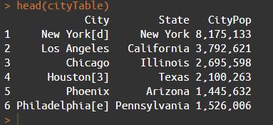
We’re getting there, but there’s still the issue of Wikipedia references in the data. Notice New York, Houston, and Philadelphia are followed by brackets.

We can use the gsub() function to remove these.

cityTable$City <- gsub("\\[.*","",cityTable$City)

Basically what we’re doing here is searching the City column for any instances of an opening bracket and deleting it and anything that follows from the string. Using head() again shows us this seems to have worked.

Now that we have our city data table ready to go we can narrow it down to only the cities we care about.

# Selecting only the cities with people names.
cityTableNames <- subset(cityTable, City %in% cities)

Well something hasn’t worked. Our list of ten cities has been cut down to three. This is because we were looking for a perfect match. Austin, Charlotte, and Jackson are the only cities that matched exactly what was in our cities variable. cities contains Antonio and Jose for example, that weren’t picked up because the cities are San Antonio and San Jose. There may be a more elegant solution, but I think it’s time for a loop.

For loops

Before starting our loops, I’m going to clear out the cityTableNames dataframe we just created. I’ll be using it again and this is just to ensure the three cities that previously made it in are not duplicated.

# Empty our df so we don't duplicate the three that worked above
cityTableNames <- data.frame(City = as.character(character()), 
                             State = as.character(character()),
                             CityPop = as.character(character()))

So, let’s break out what we want to do one step at a time.

• Look at each city in cityTable
• Compare it to each element in our list of cities.
• If there’s a match, add it to cityTableNames
• If not, keep going.

This doesn’t seem too bad. To look at each city in city table we can open up a for loop.

for (i in 1:length(cityTable[,1])) {

And since we want to compare it against each item of our list of cities, let’s use a for loop for that too.

for (i in 1:length(cityTable[,1])) {                                  
  for (j in cities) {                                                 

For the sake of checking if this is working, I’ll have the loop print the comparison it’s making every time it iterates to the console . I’ll also include a 0.5 second delay between iterations so we can see the output.

for (i in 1:length(cityTable[,1])) {                                   
  for (j in cities) {                                                  
    print(paste0(cityTable[i,1]," - ", j))      # Prints the name of the city and the name we're checking                                          
    Sys.sleep(0.5)   

So how do we check if the city name is in our cities variable? R has a few options in pattern matching. We’ll be using grepl() to check for a match, since it returns a boolean value. Let’s print our grepl() above our Sys.sleep() line in our code and see what happens. For now, we’re only printing; we get a TRUE or FALSE in the console we can use to determine if our code will work.

for (i in 1:length(cityTable[,1])) {                                   
  for (j in cities) {                                                  
    print(paste0(cityTable[i,1]," - ", j))      # Prints the name of the city and the name we're checking 
    print(grepl(pattern = j, cityTable[i,1]))   # Pattern is name of city, second argument is where to look for it.                                     
    Sys.sleep(0.5)   

Looking at San Antonio we can see it’s returning TRUE when comparing it to the name Antonio from our list. Skimming through the output it looks like this is working for all of our cities, so let’s add an if statement to generate a new dataframe containing only the cities we need.

for (i in 1:length(cityTable[,1])) {                                   
  for (j in cities) {                                                  
    print(paste0(cityTable[i,1]," - ", j))      # Prints the name of the city and the name we're checking 
    print(grepl(pattern = j, cityTable[i,1]))   # Pattern is name of city, second argument is where to look for it.                                     
    # Sys.sleep(0.5)                            # Comment out Sys.sleep when running loop for real.
    if (grepl(pattern = j, cityTable[i,1])) {   
      cityTableNames <- rbind(cityTableNames,cityTable[i,])
    }
  }
}

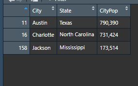
Let’s see what that gave us with View(cityTableNames).

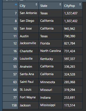
Looks good, but from our ten names we have 13 results. No problem, the name Jackson gave us two cities: Jackson MS, and Jacksonville FL. We also got two for Ana – Santa Ana CA, and Anaheim CA. While Anaheim is named after the Santa Ana River, I won’t be taking it – it just doesn’t look like a name the way the rest do. Removing it is easy enough.

cityTableNames <- cityTableNames[cityTableNames$City != "Anaheim",]

Combining the two datasets

We now have two variables – cityTableNames, with info on our cities and their populations, and groupedNames, with the names and the number of people. Now all we need to do is combine them into one dataframe. I’ll start by adding two empty columns to cityTableNames that will hold the name data.

cityTableNames <- cbind(cityTableNames, Name = "", PeopleWithName = "", stringsAsFactors = F)

In order to add the names and amounts we’ll use our nested loops again. Firstly, we’re checking the name of every city in our dataframe, so opening our loop looks like this:

for (city in cityTableNames$City) {

We want to check this against every city in our list as we did above.

for (city in cityTableNames$City) {
  for (x in cities) {

Same as we did in our previous loops, we’ll be using grepl() to determine if the word we’re looking for is contained in the name of the city. Again we can test this by printing. Let’s print the name of the city, the name we’re checking, and the result of our grepl().

for (city in cityTableNames$City) {
  for (x in cities) {
    print(paste0(city, " - ", x, " ---", grepl(pattern = x, city)))
    Sys.sleep(0.1)

This time we can see for San Jose we are getting TRUE only on Jose – so we know this is working. We can complete our loop by adding an if statement. If our grepl() returns TRUE, add the details of that name to columns 4 and 5 of our dataset (remember, R indexes starting at 1).

for (city in cityTableNames$City) {
  for (x in cities) {
    print(paste0(city, " - ", x, " ---", grepl(pattern = x, city)))
    Sys.sleep(0.1)
    if (grepl(pattern = x, city)) {
      cityTableNames[cityTableNames$City == city, 4] <- as.character(x)
      cityTableNames[cityTableNames$City == city, 5] <- as.integer(groupedNames[groupedNames$Name == x,2])
    }
  }
}

Now lets View() our updated table!

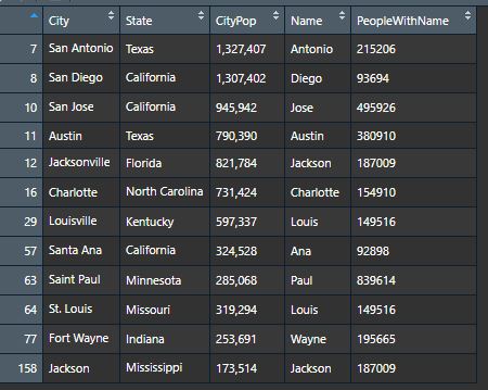
So we have our numbers, now we’re nearly ready to do some maths on them. Notice anything strange about the two number columns? Our CityPop column has a comma as a thousands separator, but our PeopleWithName column doesn’t. That’s because when we took our CityPop column from Wikipedia – we took it exactly as it appeared. We took is as a character. To perform mathematical operations on it, we need to change it to an integer. If we jump straight in and use as.integer() immediately, those commas will hurt us – we’ll end up with all NAs. as.integer() will only work once we’ve removed those commas. For this we’ll use gsub().

cityTableNames$CityPop <- gsub(",","",cityTableNames$CityPop)           # Replaces "," with nothing

Now we’re safe to change the data type for our CityPop column. We’ll change our PeopleWithName column too.

cityTableNames$CityPop <- as.integer(cityTableNames$CityPop)
class(cityTableNames$CityPop)  

cityTableNames$PeopleWithName <- as.integer(cityTableNames$PeopleWithName)
class(cityTableNames$PeopleWithName)

Finally, let’s add one more column showing us the difference , and then sort the dataframe by that difference using the order() function.

cityTableNames <- cbind(cityTableNames, Difference = cityTableNames$CityPop - cityTableNames$PeopleWithName)
cityTableNames <- cityTableNames[order(-cityTableNames$Difference),]

Now we can view our final table.

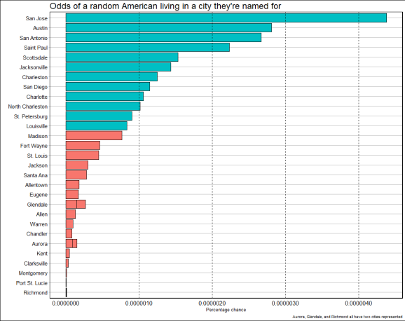
Let’s throw this into a plot to make it a bit nicer to read.

Let’s add in some more cities and see how we get on.

What did we learn?

Well… cities are big; there’s not a lot of people called Diego in the States; and there’s almost exactly the same amount of Jacksons as there are people in Jackson Mississippi.

Most importantly though, we learned that if you pick an American at random there’s about a 0.000004% chance that they are named Diego AND live in San Diego.