
A shinny app to compute and visualize roadkill hotspots over linear features
Want to share your content on R-bloggers? click here if you have a blog, or here if you don't.
In this post I’m going to explain how to use the package roadHotspots. This is just a development version located in github and I must say that I have no further intentions of continuing to work on this. If someone find this useful and would like to continue where I’ve left, please contact me.
I’ve created this project just to demonstrate that with some (limited) programming knowledge, free open-source tools and approximately 20h of work it’s possible to develop a useful and simple software with a user-friendly interface and a great scientific potential.
To install the package you first need devtools. Then, just run the following code:
library(devtools)
devtools::install_github("bmsasilva/roadHotspots")
This package provides a shiny app that allows to compute and visualize hotspots over linear features (eg. roads) for a set of observations (eg. animal crossings, roadkills). I’ve just implemented two computation algorithms, Gaussian kernel density estimation and Malo’s method (Malo et al. 2004). As I said before this is just a proof of concept and it’s not really my area of expertise. I know that there are more advanced hotspot calculation algorithms but I’ll let that for the experts in this field. To start the app just do:
run_app()
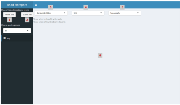
Now that you have the app running you will see a series of buttons and drop down menus. On the top right corner you have two buttons to access the file system (indicated in the image by the gray boxes 1 and 2) to choose the data for the app to work. You must select 2 files: a shapefile with the roads you’re analyzing and a csv file with roadkills/observations. The csv must have three columns: species id, X_coord and Y_coord, by this order. The coordinate system of the shapefile is irrelevant, but the coordinate system used in the csv must be the same.
The drop down menus indicated by the gray boxes 3 and 4 allow to choose some features for the implemented algorithms. Box 3 is for the bandwidth size for the density kernel and box 4 is for the probability of Malo’s method, which is based on a Poisson distribution. The drop down indicated by box 5 is to select the type of map for visualization. Finally, in the space indicated by box 6 the map with the respective density kernel or hotspot segments (I’ve decided to use 500m segments) are indicated.
The packages comes with some sample data for testing. To find the location of these files run:
system.file("extdata", package = "roadHotspots")
After importing the data into the app you will get the algorithms computed and ready for visualization. From the below picture you can see that the water course near the town “Parvoíce” is the one with the greatest density of roadkils/observations.
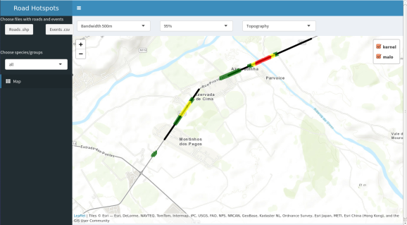
By default the topography map is loaded with both the Malo’s method and the kernel density hotspot algorithms loaded. The kernel is recoded into 3 classes, red, yellow and green (being red the most dense). For Malo’s method the black road segments are the most dense ones. In the check boxes on the top right you can select the method you want to see. Also you can change the map view aswell. Below image shows the topographic view.

So, in conclusion: you don’t need ninja programming skills nor absurd funding to create useful and easy to use softwares. With a bit of motivation and a few hours of work a lot can be achieved nowadays.
Just a cautionary note: all of this was done with free software and I don’t guarantee that it will work in Windows.
R-bloggers.com offers daily e-mail updates about R news and tutorials about learning R and many other topics. Click here if you're looking to post or find an R/data-science job.
Want to share your content on R-bloggers? click here if you have a blog, or here if you don't.