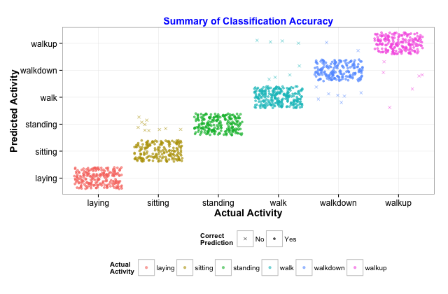
This is one of my favorite charts, it easily allows one to see how many predictions are right, and it allows one to see where the wrong ones are as well. It is the equivalent of a confusion matrix, but sometimes a picture is worth a thousand words. Some sample code is included below.

    This program is free software: you can redistribute it and/or modify
    it under the terms of the GNU General Public License as published by
    the Free Software Foundation, either version 3 of the License, or
    (at your option) any later version.

    This program is distributed in the hope that it will be useful,
    but WITHOUT ANY WARRANTY; without even the implied warranty of
    MERCHANTABILITY or FITNESS FOR A PARTICULAR PURPOSE.  See the
    GNU General Public License for more details.

    <http://www.gnu.org/licenses/>.
    Developed by Mario Segal

#requires ggplot2. Data has to be in a dataset with three columns: actual, predicted and match.
#match is Yes if actual and predicted match, No otherwise.

require(ggplot2)

fitchart <- ggplot(chartdata,aes(x=actual,y=predicted,color=actual,shape=match))+geom_jitter(alpha=.6)+theme_bw()
fitchart <- fitchart + ylab(“Predicted Activity”)+xlab(“Actual Activity”)+ggtitle(“Summary of Classification Accuracy”)
fitchart <- fitchart+theme(legend.position=”bottom”)+theme(plot.title = element_text(size=14,color=”blue”, face=”bold”))
fitchart <- fitchart+theme(axis.title.x = element_text(face=”bold”,size=14),axis.title.y = element_text(face=”bold”,size=14))
fitchart <- fitchart+theme(axis.text.x=element_text(angle=0,color=”black”,size=12),axis.text.y=element_text(color=”black”,size=12))
fitchart <- fitchart + theme(legend.text = element_text(colour=”black”, size = 10),legend.title = element_text( face=”bold”))
fitchart <- fitchart + scale_color_discrete(name=”Actual\nActivity”)+scale_shape_manual(values=c(4,20),name=”Correct\nPrediction”)
fitchart