
A Note on the Dirichlet Distribution
Want to share your content on R-bloggers? click here if you have a blog, or here if you don't.
In 1839, the gifted mathematician Peter Gustav Lejeune Dirichlet was attached to the Philosophy department at the University of Berlin working for less than full pay even though he had become a member of the Prussian Academy of Sciences in 1832. At that time, to become a “full professor” at the university it was required that a candidate deliver a Habilitationsschrift lecture in Latin. Apparently, Dirichlet’s facility with Latin wasn’t up to the task, so like many proficient “adjunct professors” today, Dirichlet took a side gig to support his family. He taught math at a military school. Anyway, I digress. It was about that time that Dirichlet began to work on a problem in celestial mechanics which involved this integral:
![]()
Here ![]() which is attracted to a point
which is attracted to a point ![]() where
where ![]() is the force of attraction
is the force of attraction ![]() and
and ![]() is the Euclidean norm.
is the Euclidean norm.
After a supernaturally insightful series manipulations detailed by Gupta and Richards, Dirichlet arrived at the following integral
![]() which you will recognize as the Beta function, the normalizing constant for the Dirichlet distribution:
which you will recognize as the Beta function, the normalizing constant for the Dirichlet distribution:
![]()
with mean ![]() and variance
and variance ![]()
where
![]() and
and ![]()
The Dirichlet distribution is a multivariate generalization of the Beta distribution that is often used in Bayesian statistics as a prior distribution for categorical and multinomial distributions. I illustrated this use of the Dirichlet in a previous post while constructing a Bayesian model for a three-state Markov chain. The Dirichlet distribution is remarkable in that it brings together 18th and 19th century work in analysis as exemplified by the Gamma, Beta and digamma functions with early 20th ideas from geometry and topology (the simplex) and modern Bayesian statistics.
The (2)-Simplex
A simplex is a generalization of the notion of a triangle to multiple dimensions. Informally in K dimensions, a simplex is the simplest polygon that is the convex hull of its K vertices. The vectors that comprise the simplex must be non-negative and sum to 1. So, a simplex is a natural way to represent probabilities that sum to 1 in multidimensional spaces.
The support for the three dimensional Dirichlet distribution, the points on which the distribution is defined, is a (2)-simplex the triangular subset of a 2-dimensional plane intersecting the Euclidean axes at the points (1,0,0), (0,1,0), and (0,0,1). (Orient the triangle in the interactive plot below so that the reference plane is on top and the tip is pointing downward and you will see how the axes line up.)
R packages used in this post
library(ggplot2)
library(gganimate)
library(dplyr)
library(magick)
library(MCMCpack)  # for rdirichlet
library(gtools)  # for ddirichlet
#library(patchwork)  # for combining plots
library(threejs)
library(extraDistr)
Show the code
set.seed(42)

# Sample from Dirichlet distribution over 3 categories
n_samples <- 2000
alpha <- c(1, 1, 1)  # uniform prior over the simplex
samples <- rdirichlet(n_samples, alpha)

# 3D coordinates: each row is (x, y, z)
x <- samples[,1]
y <- samples[,2]
z <- samples[,3]

# Visualize using threejs scatterplot
scatterplot3js(x = x, y = y, z = z,
               color = "steelblue",
               size = 0.2,
               bg = "black",
               main = "2-simplex",
               axisLabels = c(
                 "(1,0,0)",
                 "(0,1,0)",
                 "(0,0,1)"
               ))
When ![]() , the Dirichlet density is symmetric about the middle of the simplex,
, the Dirichlet density is symmetric about the middle of the simplex, ![]() . In the special case when
. In the special case when ![]() , the density is uniform over the simplex. When all the
, the density is uniform over the simplex. When all the ![]() the density is concentrated at the vertices of the simplex, and when
the density is concentrated at the vertices of the simplex, and when ![]() , the density is concentrated in the center of the simplex with most of the mass concentrated on a few values.
, the density is concentrated in the center of the simplex with most of the mass concentrated on a few values.
How the symetric Dirichlet distribution changes as  changes
The following animation, which projects the above plot onto two dimensions, shows how the Dirichlet distribution changes as the common value of ![]() , called the concentration parameter, moves systematically from (1,1,1), the uniform distribution, to (0.1,0.1,0.1).
, called the concentration parameter, moves systematically from (1,1,1), the uniform distribution, to (0.1,0.1,0.1).
Code for helper functions
# This function generates the data frame for the animation
generate_dirichlet_animation_data <- function(alpha1_values, alpha2_values, alpha3_values, n_samples = 2000) {
  library(MCMCpack)

  # Triangle vertices
  v1 <- c(1, 0)
  v2 <- c(0, 1)
  v3 <- c(0, 0)

  # Projection function
  project_to_triangle <- function(x1, x2, x3) {
    x <- x1 * v1[1] + x2 * v2[1] + x3 * v3[1]
    y <- x1 * v1[2] + x2 * v2[2] + x3 * v3[2]
    data.frame(x = x, y = y)
  }

  # Generate animation data
  animation_data <- do.call(rbind, lapply(seq_along(alpha1_values), function(i) {
    alpha <- c(alpha1_values[i], alpha2_values[i], alpha3_values[i])
    samples <- rdirichlet(n_samples, alpha)
    projected <- project_to_triangle(samples[,1], samples[,2], samples[,3])
    projected$alpha1 <- alpha[1]
    projected$alpha2 <- alpha[2]
    projected$alpha3 <- alpha[3]
    projected$frame <- i
    projected
  }))

  return(animation_data)
}

# This function creates the animated plot
plot_dirichlet_evolution <- function(animation_data) {
  library(ggplot2)
  library(gganimate)
  library(grid)  # for arrow units

  # Triangle vertices
  v1 <- c(1, 0)
  v2 <- c(0, 1)
  v3 <- c(0, 0)

  # Label positions
  label_df <- data.frame(
    x = c(v1[1], v2[1], v3[1]),
    y = c(v1[2], v2[2], v3[2]),
    label = c("(1,0,0)", "(0,1,0)", "(0,0,1)"),
    nudge_x = c(-0.08, 0.1, 0),
    nudge_y = c(0, 0, 0.08)
  )

  # Triangle outline
  triangle_df <- data.frame(
    x = c(v1[1], v2[1], v3[1], v1[1]),
    y = c(v1[2], v2[2], v3[2], v1[2])
  )

  # Build plot
  p_animation <- ggplot(animation_data, aes(x = x, y = y)) +
    geom_point(alpha = 0.3, size = 0.8, color = "steelblue") +
    geom_density_2d(color = "red", alpha = 0.7) +
    geom_path(data = triangle_df, aes(x = x, y = y), color = "black", size = 1) +
    annotate("segment", x = 1, y = 0, xend = 0, yend = 1,
             arrow = arrow(length = unit(0.2, "cm")),
             color = "darkgreen", size = 1.2) +
    xlim(0, 1) + ylim(0, 1) +
    geom_text(data = label_df,
              aes(x = x, y = y, label = label),
              nudge_x = label_df$nudge_x,
              nudge_y = label_df$nudge_y,
              size = 4, fontface = "bold", color = "black") +
    labs(
      title = "Dirichlet Prior Evolution",
      subtitle = "",
      x = "Projected X",
      y = "Projected Y",
      caption = "Transition from uniform to concentrated distribution"
    ) +
    theme_minimal() +
    theme(
      plot.title = element_text(size = 16, hjust = 0.5),
      plot.subtitle = element_text(size = 14, hjust = 0.5),
      axis.title = element_text(size = 12),
      plot.caption = element_text(size = 10, hjust = 0.5)
    ) +
    transition_states(frame,
                      transition_length = 1,
                      state_length = 2) +
    ease_aes('sine-in-out')

  return(p_animation)
}

#| message: false
#| warning: false
#| code-fold: true
#| code-summary: "Animation Code"
#|
set.seed(42)

# Parameters
alpha1_values <- seq(1, 0.1, by = -0.01)  # starts high, ends low
alpha2_values <- seq(1, 0.1, by = -0.01)   # starts low, ends high
alpha3_values <- seq(1, 0.1, by = -0.01)   # starts low, ends high

animation_data <- generate_dirichlet_animation_data(alpha1 = alpha1_values,
                                                    alpha2 = alpha2_values,
                                                    alpha3 = alpha3_values,
                                                    n_samples = 2000)

plot_dirichlet_evolution(animation_data)
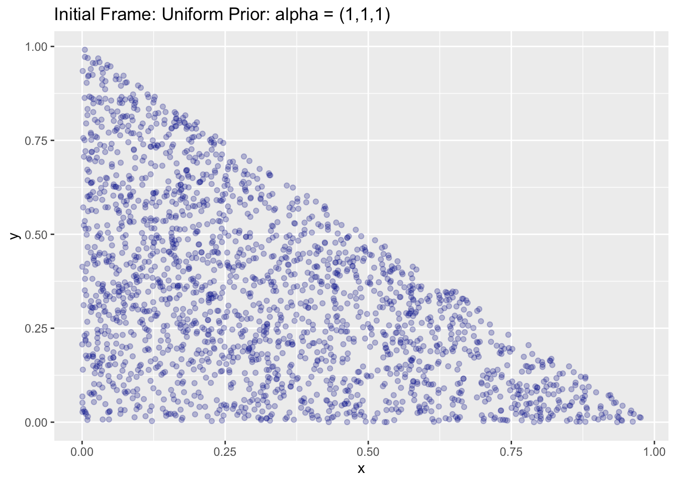
These next two plots, the first and last frames of the animation, clearly show how the density moves from being uniformly distributed over the simplex to being concentrated at the vertices of the simplex. When modeling the development of a multi-state Markov chain, as I was doing in the post I alluded to above, it is common practice to select a uniform Dirichlet prior with ![]() . However, if you believe that the process is likely to start off uniformly distributed among the states, then a prior with
. However, if you believe that the process is likely to start off uniformly distributed among the states, then a prior with ![]() might be appropriate. If you had reason to believe that the process would start off concentrated on particular states, then you might explore using an asymmetric distribution by setting different values for the
might be appropriate. If you had reason to believe that the process would start off concentrated on particular states, then you might explore using an asymmetric distribution by setting different values for the ![]() . The code driving these animations might be helpful.
. The code driving these animations might be helpful.
Show the code
ggplot(subset(animation_data, frame == 1), aes(x = x, y = y)) +
  geom_point(alpha = 0.3, color = "darkblue") +
  ggtitle("Initial Frame: Uniform Prior: alpha = (1,1,1)")
Show the code
  ggplot(subset(animation_data, frame == max(animation_data$frame)), aes(x = x, y = y)) +
  geom_point(alpha = 0.3, color = "red") +
  ggtitle("Final Frame: Concetrated Prior: alpha = (.1,.1,.1)")

This concentration of density as ![]() increases is very apparent in this next simulation as
increases is very apparent in this next simulation as ![]() moves from (0.1, 0.1, 0.1) to (10.0, 10.0, 10.0). Here we see the distribution concentrating on the mean,
moves from (0.1, 0.1, 0.1) to (10.0, 10.0, 10.0). Here we see the distribution concentrating on the mean, ![]() = (1/3, 1/3, 1/3).
= (1/3, 1/3, 1/3).
Show the code
#Define alpha trajectories
alpha1 <- seq(.1, 10, by = 0.1)
alpha2 <- seq(.1, 10, by = 0.1)
alpha3 <- seq(.1, 10, by = 0.1)

animation_data <- generate_dirichlet_animation_data(alpha1, alpha2, alpha3, n_samples = 2000)

anim2 <- plot_dirichlet_evolution(animation_data)
anim2
Note that the animation ![]() passes through (0.5, 0.5, 0.5) which is the Jeffreys prior for the Dirichlet distribution.
passes through (0.5, 0.5, 0.5) which is the Jeffreys prior for the Dirichlet distribution.
Variance and Differential Entropy
The Wikipedia article for the Dirichlet distribution prominently displays the distribution’s differential entropy:
![]()
where ![]() and
and ![]() are defined above and
are defined above and ![]() is the digamma function. (This equation triggered my mention of the digamma function above.) But please be advised that differential entropy defined as:
is the digamma function. (This equation triggered my mention of the digamma function above.) But please be advised that differential entropy defined as: ![]() for continuous distributions is not the same as the Shannon entropy
for continuous distributions is not the same as the Shannon entropy ![]() for discrete distributions and does not have a similar interpretation. Among other things, differential entropy can be negative, in not invariant under a change of variables, and probably doesn’t conform to any intuition you may have developed about maximum entropy. The plot on the left below shows the behavior of the differential entropy for the symmetric Dirichlet distribution we have been considering as
for discrete distributions and does not have a similar interpretation. Among other things, differential entropy can be negative, in not invariant under a change of variables, and probably doesn’t conform to any intuition you may have developed about maximum entropy. The plot on the left below shows the behavior of the differential entropy for the symmetric Dirichlet distribution we have been considering as ![]() moves from (0.1, 0.1, 0.1) to (5.0, 5.0, 5.0). Note that the entropy keeps increasing beyond the point
moves from (0.1, 0.1, 0.1) to (5.0, 5.0, 5.0). Note that the entropy keeps increasing beyond the point ![]() which corresponds to the uniform distribution over the simplex.
which corresponds to the uniform distribution over the simplex.
Show the code
# Define the number of dimensions for the symmetric Dirichlet distribution
n <- 3

# Define a function to calculate the entropy of a symmetric Dirichlet distribution
dirichlet_entropy <- function(alpha, n) {
  # This formula is for a symmetric Dirichlet distribution
  # where all parameters a_i are equal to alpha.
  # The formula uses the digamma function (psi) and the log-gamma function (lgamma).
  # H(alpha) = log(Beta(alpha)) + (n * alpha - n) * psi(n * alpha) - n * (alpha - 1) * psi(alpha)
  # log(Beta(alpha)) = n * lgamma(alpha) - lgamma(n * alpha)
  # The final formula is simplified for symmetric case.

  # lgamma(x) is the log-gamma function
  # digamma(x) is the psi function, the first derivative of lgamma(x)

  entropy_val <- lgamma(n * alpha) - n * lgamma(alpha) +
                 (n * alpha - n) * digamma(n * alpha) -
                 n * (alpha - 1) * digamma(alpha)

  return(entropy_val)
}

# Create a sequence of alpha values from 0.1 to 5
alpha_values <- seq(0.1, 5, by = 0.01)

# Calculate the entropy for each alpha value
entropy_values <- sapply(alpha_values, dirichlet_entropy, n = n)

# Create a data frame for plotting
plot_data <- data.frame(alpha = alpha_values, entropy = entropy_values)

# Plot the entropy values
ggplot(plot_data, aes(x = alpha, y = entropy)) +
  geom_line(size = 1.2, color = "steelblue") +
  labs(
    title = "Entropy of a Symmetric Dirichlet Distribution",
    subtitle = paste("for n =", n, "dimensions"),
    x = "Alpha (Concentration Parameter)",
    y = "Entropy"
  ) +
  geom_vline(xintercept = 1, linetype = "dashed", color = "red", size = 1) +
  annotate("text", x = 1.1, y = max(entropy_values) * 0.9,
           label = "Alpha = 1 (Uniform Distribution)",
           color = "red", hjust = 0, size = 4) +
  theme_minimal(base_size = 14) +
  theme(plot.title = element_text(hjust = 0.5),
        plot.subtitle = element_text(hjust = 0.5))

Show the code
k <- seq(.1, 10, by = 0.1)

mean_dir <- numeric(length(k))
var_dir <- numeric(length(k))
for (i in seq_along(k)) {
  alpha <- k[i]
  sum_alpha <- alpha * 3
  mean_dir[i] <- alpha / sum_alpha
  var_dir[i] <- (alpha * (sum_alpha - alpha)) / (sum_alpha^2 * (sum_alpha + 1))
}
df <- data.frame(k = k, mean = mean_dir, variance = var_dir)
ggplot(df, aes(x = k, y = variance)) +
  geom_line(color = "blue", size = 1) +
  labs(
    title = "Variance of Dirichlet Distribution vs Alpha Parameter",
    x = "Alpha Parameter (k)",
    y = "Variance"
  )

The plot on the right shows the variance of the Dirichlet distribution as a function increasing ![]() . We see that the variance decreases towards zero as
. We see that the variance decreases towards zero as ![]() increases. This is reflected in the second animation above which shows the distribution concentrating on the mean. Uncertainty is going to zero but differential entropy is shooting off towards to infinity. If you are nevertheless intrigued by differential entropy, you may want to have a look at the references I have included below.
increases. This is reflected in the second animation above which shows the distribution concentrating on the mean. Uncertainty is going to zero but differential entropy is shooting off towards to infinity. If you are nevertheless intrigued by differential entropy, you may want to have a look at the references I have included below.
References
Bela A. Frigyik, Amol Kapila, and Maya R. Gupta, Introduction to the Dirichlet Distribution and Related Processes
Thomas M. Cover and Joy A. Thomas, Elements of Information Theory, Wiley-Interscience Edition: 2nd Edition, (2006)
Rameshwar Gupta and Donald St. P. Richards, The History of the Dirchet and Liouville Distributions international Statistical Review (2001)
Jiayu Lin, On the Dirichlet Distribution
R-bloggers.com offers daily e-mail updates about R news and tutorials about learning R and many other topics. Click here if you're looking to post or find an R/data-science job.
Want to share your content on R-bloggers? click here if you have a blog, or here if you don't.