Sample

The 2024 sample was designed to represent U.S. citizens age 18 or older. Respondents were recruited from both in-person and web samples, with careful notes on eligibility and exclusions.

Codebook

The codebook decodes variable names into something human-readable.

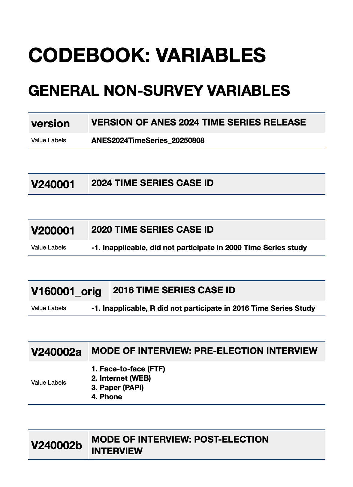
Here are two variables we’ll use:

• V240002b: MODE OF INTERVIEW: POST-ELECTION: This variable captures the mode in which the respondent completed the majority of the post-election survey.
  • -7. Insufficient parital, interview deleted
  • -6. No post interview
  • 1. Face-to-face (FTF)
  • 2. Internet (WEB)
  • 3. Paper (PAPI)
  • 4. Phone
  • 5. Video
• V241229: PRE: HOW OFTEN TRUST GOVERNMENT IN WASHINGTON TO DO WHAT IS RIGHT [REVISED]:
  • -9. Refused
  • -8. Don’t know
  • -1. Inapplicable
  • 1. Always
  • 2. Most of the time
  • 3. About half the time
  • 4. Some of the time
  • 5. Never

Let’s recode V241229 for easier analysis:

anes_2024_code <-
  anes_2024 |> 
  mutate(
    TrustGovernment = factor(
      case_when(
        V241229 == 1 ~ "Always",
        V241229 == 2 ~ "Most of the time",
        V241229 == 3 ~ "About half the time",
        V241229 == 4 ~ "Some of the time",
        V241229 == 5 ~ "Never",
        .default = NA
      ),
      levels = c("Always", "Most of the time", "About half the time", "Some of the time", "Never")
    )
  )

See more on codebooks.

Finding the right weight

The ANES documentation lists which weight variables go with which sample:

Since we’re looking at the post-election fresh in-person sample, we’ll use weight variable V240101b.

One important note: ANES weights add up to the sample size, not the population size. Let’s confirm:

anes_2024_code |> filter(V240101b > 0) |> summarize(sum = sum(V240101b))

# A tibble: 1 × 1
    sum
  <dbl>
1   925

This matches the 925 respondents shown in the documentation’s sample table.

Adjusting for the population

If we want to make inferences about the entire U.S. population, we need to adjust the weights. The target population for this sample is about 232.5 million U.S. citizens aged 18 or older, but that’s just a rough number. Per the documentation, for something more precise, we can pull population counts from the 2023 American Community Survey 1-year estimates.

Thank you, Stephanie, for writing up the code for the population estimates!

library(tidycensus)

varlist_2023 <- load_variables(2023, "acs1")

citizen_pop_18_plus <-
  get_acs(
    geography = "state",
    variable = "S2901_C01_001",
    year = 2023,
    survey = "acs1"
  )

pums_vars_2023 <- pums_variables |>
  as_tibble() |>
  filter(year == 2023, survey == "acs1")

pums_vars_2023 |>
  filter(var_code %in% c("AGEP", "TYPEHUGQ", "CIT")) |>
  select(var_code, var_label, val_min, val_max, val_label) |>
  print(n = 50)

# Find those who are 18+ and in group quarters
get_citizen_pop_18_plus_gq <- function(state) {
  get_pums(
    variables = c("AGEP", "TYPEHUGQ"),
    state = state,
    year = 2023,
    survey = "acs1",
    variables_filter = list(
      TYPEHUGQ = 2:3 ,
      CIT = 1:4,
      AGEP = (18:200)
    )
  ) |>
    summarize(estimate = sum(PWGTP), .by = STATE)
}

citizen_pop_18_plus_gq_l <- c(state.abb, "DC") |>
  map(get_citizen_pop_18_plus_gq)

citizen_pop_18_plus_gq_df <-
  citizen_pop_18_plus_gq_l |>
  list_rbind() |>
  rename(estimate_gq = estimate)

state_pops <- citizen_pop_18_plus |>
  select(GEOID, NAME, estimate_tot = estimate) |>
  full_join(citizen_pop_18_plus_gq_df, by = c("GEOID" = "STATE")) |>
  filter(NAME != "Puerto Rico") |>
  mutate(estimate_scope = estimate_tot - estimate_gq)

# Total without AK and HI
targetpop <-
  state_pops |>
  filter(!GEOID %in% c("02", "15")) |>
  summarize(TargetPop = sum(estimate_scope))

# Total with AK and HI
state_pops |>
  summarize(TargetPop = sum(estimate_scope))

The estimated target population (targetpop) for 2024 is 232,449,541. Now we can rescale the ANES weights so they add up to the population size:

anes_adjwgt <- anes_2024_code |>
  mutate(Weight = V240101b / sum(V240101b, na.rm = TRUE) * targetpop)

Strata and clusters

The documentation also tells us which strata and PSU (cluster) variables pair with each weight.

For V240101b, those are:

• Strata: V240101d
• PSU: V240101c

More on sampling design can be found in this chapter.

Putting it all together

Finally, we can build the design object. We’ll also filter to respondents who actually completed the in-person post-election interview (V240002b == 1):

options(survey.lonely.psu = "adjust")

anes_des <- anes_adjwgt |>
  filter(V240002b == 1) |>
  as_survey_design(
    weights = Weight,
    strata = V240101d,
    ids = V240101c,
    nest = TRUE
  )

anes_des

And there we go! anes_des is our fully specified survey design object. From here on, we use it so every estimate we calculate properly reflects the survey’s design.