Note: This post was inspired by the “Classroom Bingo” probability puzzle in the Royal Statistical Society’s Significance magazine (Dec 2021 edition).

Set-up

Imagine that we are playing bingo, but where the numbers are generated by the roll of two 6-sided dice with faces 1, 2, …, 6. Each round, the two dice are rolled. If the sum of the two dice appears on your bingo card, you can strike it off. The game ends when you strike off all the numbers on your card.

For this simple game, you are asked to write just two numbers on your bingo card (which can be the same number if you wish). What two numbers should you write in order to finish the game as quickly as possible (on average)?

Intuition

With the roll of two dice, the most probable outcome is 7 (6 out of 36), followed by 6 and 8 (5 out of 36), and so on. Hence, the two numbers you should write down are probably (7, 7) or (7, 6) / (7, 8). Which is better?

Simulation

This problem space is small enough that we can estimate the number of rounds for each possible bingo card via Monte Carlo simulation. Here is the function that runs one round of dice bingo in R:

# Roll `nDice` dice with sides 1, 2, ..., `nFaces` and return the sum
RollDice <- function(nDice, nFaces) {
  dice <- sample(nFaces, size = nDice, replace = TRUE)
  sum(dice)
}

SimulateBingo <- function(bingoVec, nDice, nFaces, verbose = FALSE) {
  nRolls <- 0
  while (length(bingoVec) > 0) {
    nRolls <- nRolls + 1
    currentRoll <- RollDice(nDice, nFaces)
    
    # check if roll matches a number on card; if so, remove that number
    matchIndex <- match(currentRoll, bingoVec)
    if (!is.na(matchIndex))
      bingoVec <- bingoVec[-matchIndex]
    
    if (verbose) print(paste0("Roll ", nRolls, ": ", currentRoll, ", (", 
                              paste(bingoVec, collapse = ","), 
                              ") remaining"))
  }
  nRolls
}

The SimulateBingo function is flexible enough for us to have any number of numbers on our bingo card at the beginning of the game. Here’s an example output from SimulateBingo(), where we have 3 numbers (6, 6, 7) on our card at the beginning, and at each round we roll 2 dice with sides 1 to 6:

set.seed(2)
SimulateBingo(c(6, 6, 7), 2, 6, verbose = TRUE)

# [1] "Roll 1: 11, (6,6,7) remaining"
# [1] "Roll 2: 7, (6,6) remaining"
# [1] "Roll 3: 6, (6) remaining"
# [1] "Roll 4: 9, (6) remaining"
# [1] "Roll 5: 3, (6) remaining"
# [1] "Roll 6: 4, (6) remaining"
# [1] "Roll 7: 9, (6) remaining"
# [1] "Roll 8: 5, (6) remaining"
# [1] "Roll 9: 7, (6) remaining"
# [1] "Roll 10: 5, (6) remaining"
# [1] "Roll 11: 9, (6) remaining"
# [1] "Roll 12: 7, (6) remaining"
# [1] "Roll 13: 11, (6) remaining"
# [1] "Roll 14: 9, (6) remaining"
# [1] "Roll 15: 6, () remaining"
# [1] 15

Next, we introduce a function that runs SimulateBingo() multiple times and returns the mean number of rounds needed to complete the game:

EstimateRounds <- function(nSim, bingoVec, nDice, nFaces) {
  rounds <- replicate(nSim, SimulateBingo(bingoVec, nDice, nFaces))
  mean(rounds)
}

(For R aficionados wondering why I didn’t use ... to pass function arguments to SimulateBingo(): it’s because replicate() and ... don’t play well together. See more details here.)

The following code runs 100,000 simulations of the game for each possible pair of numbers on the bingo card (this takes a while to run):

set.seed(2)
nDice <- 2
nFaces <- 6
nSim <- 100000

df <- data.frame(matrix(nrow = 0, ncol = 3))
maxSum <- nDice * nFaces
minSum <- nDice
for (x in minSum:maxSum) {
  for (y in x:maxSum) {
    print(paste("Simulating bingoVec = (", x, ", ", y, ")"))
    meanRounds <- EstimateRounds(nSim, bingoVec = c(x, y), nDice, nFaces)
    df <- rbind(df, c(x, y, meanRounds))
  }
}
names(df) <- c("x", "y", "mean_rounds")

Let’s make a heatmap to visualize the results:

library(ggplot2)
ggplot(df, aes(factor(x), factor(y))) +
  geom_tile(aes(fill = mean_rounds)) +
  geom_text(aes(label = sprintf(mean_rounds, fmt = "%.2f"))) +
  scale_fill_distiller(palette = "Spectral") +
  labs(x = "Bingo value 1", y = "Bingo value 2", 
       title = "Mean # of dice rolls to reach bingo")
  theme_update(legend.position = "null")

Notice the symmetry in the plot: the mean number of rounds for is basically the same as that for . This makes sense due to symmetry inherent in the problem (the probability of rolling is the same as rolling for one die).

The smallest number of rounds is obtained for the pairs (6, 7) and (7, 8)!

Explanation

Let denote the number of rounds until (and including) the first time a number on the bingo card is hit, and let denote the number of rounds from then until (and including) the second number is hit. The number of rounds to complete the game is just .

Note that and are geometric random variables, and so their expectation is the reciprocal of the probability of success.

For (7, 7), the probability of success of and is the same: it’s the probability of rolling a 7, which is . Hence,

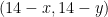
For (6, 7), the computation is a bit trickier because the distribution of depends on whether the 6 or the 7 was hit first. If 6 was hit first, then , and if 7 was hit first, then . What is the probability that 6 is hit first? It’s

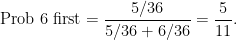
Hence,

is a geometric distribution with success probability equal to the probability that 6 or 7 is rolled, i.e. , implying that . Hence,

which is quite a bit less than the expected value for (7, 7)! (Notice that these values are very close to the simulated results.)

On second thought this makes sense: even though it takes longer to hit the second number in (6, 7), this is more than made up for in the time it takes to hit the first number, since we can hit either 6 or 7, not just 7. (Looking at the simulation results suggests that quite a few other pairs of numbers are better than (7, 7).)

Extensions

There are many interesting questions to ponder as extensions to this game:

1. What if you had to write down 3 numbers on your bingo card instead? Or 4? Or n?
2. What if there were more dice?
3. What if the dice had non-standard faces?