This post shows how to use the R packages for estimating an exclusive lasso and a group lasso. These lasso variants have a given grouping order in common but differ in how this grouping constraint is functioning when a variable selection is performed.

Lasso, Group Lasso, and Exclusive Lasso

While LASSO (least absolute shrinkage and selection operator) has many variants and extensions, our focus is on two lasso models: Group Lasso and Exclusive Lasso. Before we dive into the specifics, let’s go over the similarities and differences of these two lasso variants from the following figure.
In the above figure, 15 variables are categorized into 5 groups. Lasso selects important features irrespective of the grouping. Of course, lasso did not select Group 2’s variables but it is not intended but just an estimation result. While group lasso selects all or none in specific group, exclusive lasso selects at least one variable in each group.

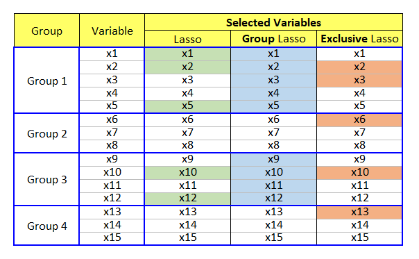
From a perspective of competition, group lasso implements a completion across groups and on the contrary, exclusive lasso makes variables in the same group compete with each other within each group.

Since we can grasp the main characteristics of two lasso modes from the above figure, let’s turn to the mathematical expressions.

Equations

There are some various expressions for these models and the next equations are for lasso, group lasso, and exclusive Lasso following Qiu et al. (2021).

\[\begin{align} \text{Lasso} &: \min \left\Vert y-X\beta \right\Vert^2 + \lambda \sum_{j=1}^{m} |\beta_j| \\ \text{Group Lasso} &: \min \left\Vert y-X\beta \right\Vert^2 + \lambda \sum_{g=1}^{G} \Vert \beta_g \Vert_2^1 \\ \text{Exclusive Lasso} &: \min \left\Vert y-X\beta \right\Vert^2 + \lambda \sum_{g=1}^{G} \Vert \beta_g \Vert_1^2 \end{align}\]
where the coefficient in \(\beta \) are divided into \(G\) groups and \(\beta_g\) denotes the coefficient vector of the \(g\)-th group.

In the group lasso, \(l_{2,1}\)-norm consists of the intra-group non-sparsity via \(l_2\)-norm and inter-group sparsity via \(l_1\)-norm. Therefore, variables of each group will be either selected or discarded entirely. Refer to Yuan and Lin (2006) for more information on the group lasso.

In exclusive lasso, \(l_{1,2}\)-norm consists of the intra-group sparsity via \(l_1\)-norm and inter-group non-sparsity via \(l_2\)-norm. Exclusive lasso selects at least one variable from each group. Refer to Zhou et al. (2010) for more information on the exclusive lasso.

R code

The following R code implements lasso, group lasso, and exclusive lasso for an artificial data set with a given group index. Required R packages are glmnet for lasso, gglasso for group lasso, and ExclusiveLasso for exclusive lasso.




The first output from the above R code is the table of coefficients of all models with given each initial \(\lambda\) parameter. We can easily find the model-specific pattern of each model.




The second output is the table of coefficients of all models with each selected lambda which is a result of cross validation.

An Interesting Property of Exclusive Lasso

As stated earlier, the exclusive lasso selects at least one variable from each group. Let’s check if this argument holds true with the next R code by setting \(\lambda\) to a higher value (100), which prevents from selecting variables.



The following result is sufficient for supporting the above explanation. While lasso and group lasso discard all variables with a higher \(\lambda\), exclusive lasso select one variable from each group. I add horizontal dotted lines for separating each group just for exposition purpose.




This is interesting and may be useful when we want to select one security in each sector when forming a diversified asset portfolio with many investment sectors. Of course, a further analysis is necessary to select arbitrary predetermined number of securities from each sector.

Concluding Remarks

This post shows how to use graoup lasso and exclusive lasso using R code. In particular, I think that the exclusive lasso delivers some interesting result which will be investigated furthermore in following research such as sector-based asset allocation (sectoral diversification).

Reference

Yuan, M. and L. Lin (2006), Model Selection and Estimation in Regression with Grouped Variables, Journal of the Royal Statistical Society, Series B 68, pp. 49–67.

Zhou, Y., R. Jin, and S. Hoi (2010), Exclusive Lasso for Multi-task Feature Selection. In International Conference on Artificial Intelligence and Statistics, pp. 988-995.

Qiu, L., Y. Qu, C. Shang, L. Yang, F. Chao, and Q. Shen (2021), Exclusive Lasso-Based k-Nearest Neighbors Classification. Neural Computing and Applications, pp. 1-15.
\(\blacksquare\)