TLDR: I’ve written an R package, cvwrapr, that helps users to cross-validate hyperparameters. The code base is largely extracted from the glmnet package. The R package is available for download from Github, and contains two vignettes which demonstrate how to use it. Comments, feedback and bug reports welcome!

Imagine yourself in the following story:

You are working on developing a supervised learning method. You ponder each detail of the algorithm day and night, obsessing over whether it does the right thing. After weeks and months of grinding away at your laptop, you finally have a fitter function that you are satisfied with. You bring it to your collaborator who says:

“Great stuff! … Now we need a function that does cross-validation for your hyperparameter.”

A wave of fatigue washes over you: weren’t you done with the project already? You galvanize yourself, thinking, “it’s not that bad: it’s just a for loop over the folds right?” You write the for loop and get a matrix of out-of-fold predictions. You now realize you have to write more code to compute the CV error. “Ok, that’s simple enough for mean-squared error…”, but then a rush of questions flood your mind:

“What about the CV standard errors? I can never remember what to divide the standard deviation by…”
“We have to compute lambda.min and lambda.1se too right?”
“What about family=’binomial’? family=’cox’?”
“Misclassification error? AUC?”

As these questions (and too much wine) make you doubt your life choices, a realization pops into your head:

“Wait: doesn’t cv.glmnet do all this already??”

And that is the backstory for the cvwrapr package, which I’ve written as a personal project.  It essentially rips out the cross-validation (CV) portion of the glmnet package and makes it more general. The R package is available for download from Github, and contains two vignettes which demonstrate how to use it. The rest of this post is a condensed version of the vignettes.

First, let’s set up some fake data.

set.seed(1)
nobs <- 100; nvars <- 10
x <- matrix(rnorm(nobs * nvars), nrow = nobs)
y <- rowSums(x[, 1:2]) + rnorm(nobs)

The lasso

The lasso is a popular regression method that induces sparsity of features in the fitted model. It comes with a hyperparmater that the user usually picks by cross-validation (CV). The glmnet package has a function cv.glmnet that does this:

library(glmnet)
glmnet_fit <- cv.glmnet(x, y)

The code snippet below shows the equivalent code using the cvwrapr package. The model-fitting function is passed to kfoldcv via the train_fun argument, while the prediction function is passed to the predict_fun argument. (See the vignette for more details on the constraints on these functions.)

library(cvwrapr)
cv_fit <- kfoldcv(x, y, train_fun = glmnet, 
                  predict_fun = predict)

The lasso with variable filtering

In some settings, we might want to exclude variables which are too sparse. For example, we may want to remove variables that are more than 80% sparse (i.e. more than 80% of observations having feature value of zero), then fit the lasso for the remaining variables.

To do CV correctly, the filtering step should be included in the CV loop as well. The functions in the glmnet package have an exclude argument where the user can specify which variables to exclude from model-fitting. Unfortunately, at the time of writing, the exclude argument can only be a vector of numbers, representing the feature columns to be excluded. Since we could be filtering out different variables in different CV folds, using the exclude argument will not work for us.

The cvwrapr package allows us to wrap the feature filtering step into the CV loop with the following code:

# filter function
filter <- function(x, ...) which(colMeans(x == 0) > 0.8)

# model training function
train_fun <- function(x, y) {
  exclude <- which(colMeans(x == 0) > 0.8)
  if (length(exclude) == 0) {
    model <- glmnet(x, y)
  } else {
    model <- glmnet(x[, -exclude, drop = FALSE], y)
  }
  return(list(lambda = model$lambda,
              exclude = exclude,
              model = model))
}

# prediction function
predict_fun <- function(object, newx, s) {
  if (length(object$exclude) == 0) {
    predict(object$model, newx = newx, s = s)
  } else {
    predict(object$model, 
            newx = newx[, -object$exclude, drop = FALSE], 
            s = s)
  }
}

set.seed(1)
cv_fit <- kfoldcv(x, y, train_fun = train_fun, 
                  predict_fun = predict_fun)

Gradient boosting: number of trees

Next, let’s look at a gradient boosting example. In gradient boosting, a common hyperparameter to cross-validate is the number of trees in the gradient boosting ensemble. The code below shows how one can achieve that with the cvwrapr and gbm packages:

library(gbm)

# lambda represents # of trees
train_fun <- function(x, y, lambda) {
  df <- data.frame(x, y)
  model <- gbm::gbm(y ~ ., data = df, 
                    n.trees = max(lambda),
                    distribution = "gaussian")
  
  return(list(lambda = lambda, model = model))
}

predict_fun <- function(object, newx, s) {
  newdf <- data.frame(newx)
  predict(object$model, newdata = newdf, n.trees = s)
}

set.seed(3)
lambda <- 1:100
cv_fit <- kfoldcv(x, y, lambda = lambda, 
                  train_fun = train_fun, 
                  predict_fun = predict_fun)

kfoldcv returns an object of class “cvobj”, which has a plot method:

plot(cv_fit, log.lambda = FALSE, xlab = "No. of trees", 
     main = "CV MSE vs. no. of trees")

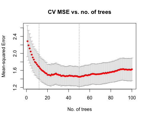
The vertical line on the right corresponds to the hyperparameter value that gives the smallest CV error, while the vertical line on the left corresponds to the value whose CV error is within one standard error of the minimum.

Computing different error metrics

Sometimes you may only have access to the out-of-fold predictions; in these cases you can use cvwrapr‘s computeError function to compute the CV error for you (a non-trivial task!).

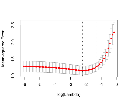
The code below does CV for the lasso with the CV error metric being the default mean squared error:

set.seed(1)
cv_fit <- kfoldcv(x, y, train_fun = glmnet, 
                  predict_fun = predict,
                  keep = TRUE)
plot(cv_fit)

What if we wanted to pick the hyperparameter according to mean absolute error instead? One way would be to call kfoldcv again with the additional argument type.measure = "mae". This would involve doing all the model-fitting again.

Since we specified keep = TRUE in the call above, cv_fit contains the out-of-fold predictions: we can do CV for mean absolute error with these predictions without refitting the models. The call below achieves that (see vignette for details on the additional arguments):

mae_err <- computeError(cv_fit$fit.preval, y, 
                        cv_fit$lambda, cv_fit$foldid, 
                        type.measure = "mae", family = "gaussian")
plot(mae_err)