Series of Azure Databricks posts:

• Dec 01: What is Azure Databricks
• Dec 02: How to get started with Azure Databricks
• Dec 03: Getting to know the workspace and Azure Databricks platform
• Dec 04: Creating your first Azure Databricks cluster
• Dec 05: Understanding Azure Databricks cluster architecture, workers, drivers and jobs
• Dec 06: Importing and storing data to Azure Databricks
• Dec 07: Starting with Databricks notebooks and loading data to DBFS
• Dec 08: Using Databricks CLI and DBFS CLI for file upload
• Dec 09: Connect to Azure Blob storage using Notebooks in Azure Databricks
• Dec 10: Using Azure Databricks Notebooks with SQL for Data engineering tasks
• Dec 11: Using Azure Databricks Notebooks with R Language for data analytics
• Dec 12: Using Azure Databricks Notebooks with Python Language for data analytics
• Dec 13: Using Python Databricks Koalas with Azure Databricks
• Dec 14: From configuration to execution of Databricks jobs
• Dec 15: Databricks Spark UI, Event Logs, Driver logs and Metrics
• Dec 16: Databricks experiments, models and MLFlow
• Dec 17: End-to-End Machine learning project in Azure Databricks
• Dec 18: Using Azure Data Factory with Azure Databricks
• Dec 19: Using Azure Data Factory with Azure Databricks for merging CSV files
• Dec 20: Orchestrating multiple notebooks with Azure Databricks
• Dec 21: Using Scala with Spark Core API in Azure Databricks
• Dec 22: Using Spark SQL and DataFrames in Azure Databricks
• Dec 23: Using Spark Streaming in Azure Databricks

Yesterday we briefly touched Spark Streaming as part of Spark component on top of Spark Core.

Another important component is Machine Learning Spark package called MLlib.

MLlib is a scalable machine learning library bringing quality algorithms and giving you process speed. (due to upgradede functionality of Hadoops’ map-reduce. Besides supporting several languages (Java, R, Scala, Python), it brings also the pipelines – for better data movement.

MLlib package brings you several covered topics:

• Basic statistics
• Pipelines and data transformation
• Classification and regression
• Clustering
• Collaborative filtering
• Frequent pattern mining
• Dimensionality reduction
• Feature selection and transformation
• Model Selection and tuning
• Evaluation metrics

The Apache Spark machine learning library (MLlib) allows data scientists to focus on their data problems and models instead of solving the complexities surrounding distributed data (such as infrastructure, configurations, and so on).

Now, let’s create a new notebook. I named mine Day24_MLlib. And select Python Language.

1.Load Data

We will use the sample data that is available in /databricks-datasets folder.

%fs ls databricks-datasets/adult/adult.data

And we will use Spark SQL to import the dataset into Spark Table:

%sql DROP TABLE IF EXISTS adult
CREATE TABLE adult (
  age DOUBLE,
  workclass STRING,
  fnlwgt DOUBLE,
  education STRING,
  education_num DOUBLE,
  marital_status STRING,
  occupation STRING,
  relationship STRING,
  race STRING,
  sex STRING,
  capital_gain DOUBLE,
  capital_loss DOUBLE,
  hours_per_week DOUBLE,
  native_country STRING,
  income STRING)
USING CSV
OPTIONS (path "/databricks-datasets/adult/adult.data", header "true")

And get the data into DataSet from Spark SQL table:

dataset = spark.table("adult")
cols = dataset.columns

2.Data Preparation

Since we are going to try algorithms like Logistic Regression, we will have to convert the categorical variables in the dataset into numeric variables.We will use one-hot encoding (and not categoy indexing)

One-Hot Encoding – converts categories into binary vectors with at most one nonzero value: Blue: [1, 0], etc.

In this dataset, we have ordinal variables like education (Preschool – Doctorate), and also nominal variables like relationship (Wife, Husband, Own-child, etc). For simplicity’s sake, we will use One-Hot Encoding to convert all categorical variables into binary vectors. It is possible here to improve prediction accuracy by converting each categorical column with an appropriate method.

Here, we will use a combination of StringIndexer and OneHotEncoder to convert the categorical variables. The OneHotEncoder will return a SparseVector.

Since we will have more than 1 stage of feature transformations, we use a Pipeline to tie the stages together; similar to chaining with R dplyr.

Predict variable will be income; binary variable with two values:

• “<=50K”
• “>50K”

All other variables will be used for feature selections.

We will be using MLlib Spark for Python to continue the work. Let’s load the packages for data pre-processing and data preparing. Pipelines for easier working with dataset and onehot encoding.

from pyspark.ml import Pipeline
from pyspark.ml.feature import OneHotEncoder, StringIndexer, VectorAssembler

We will indexes each categorical column using the StringIndexer, and then converts the indexed categories into one-hot encoded variables. The resulting output has the binary vectors appended to the end of each row.

We use the StringIndexer again to encode our labels to label indices.

categoricalColumns = ["workclass", "education", "marital_status", "occupation", "relationship", "race", "sex", "native_country"]
stages = [] # stages in our Pipeline
for categoricalCol in categoricalColumns:
    stringIndexer = StringIndexer(inputCol=categoricalCol, outputCol=categoricalCol + "Index")
    encoder = OneHotEncoder(inputCols=[stringIndexer.getOutputCol()], outputCols=[categoricalCol + "classVec"])
    stages += [stringIndexer, encoder]
    
# Convert label into label indices using the StringIndexer
label_stringIdx = StringIndexer(inputCol="income", outputCol="label")
stages += [label_stringIdx]

Use a VectorAssembler to combine all the feature columns into a single vector column. This goes for all types: numeric and one-hot encoded variables.

numericCols = ["age", "fnlwgt", "education_num", "capital_gain", "capital_loss", "hours_per_week"]
assemblerInputs = [c + "classVec" for c in categoricalColumns] + numericCols
assembler = VectorAssembler(inputCols=assemblerInputs, outputCol="features")
stages += [assembler]

3. Running Pipelines

Run the stages as a Pipeline. This puts the data through all of the feature transformations we described in a single call.

partialPipeline = Pipeline().setStages(stages)
pipelineModel = partialPipeline.fit(dataset)
preppedDataDF = pipelineModel.transform(dataset)

Now we can do a Logistic regression classification and fit the model on prepared data

from pyspark.ml.classification import LogisticRegression
# Fit model to prepped data
lrModel = LogisticRegression().fit(preppedDataDF)

And run ROC

# ROC for training data
display(lrModel, preppedDataDF, "ROC")

And check the fitted values (from the model) against the prepared dataset:

display(lrModel, preppedDataDF)

Now we can check the dataset with added labels and features:

selectedcols = ["label", "features"] + cols
dataset = preppedDataDF.select(selectedcols)
display(dataset)

4. Logistic Regression

In the Pipelines API, we are now able to perform Elastic-Net Regularization with Logistic Regression, as well as other linear methods.

from pyspark.ml.classification import LogisticRegression

# Create initial LogisticRegression model
lr = LogisticRegression(labelCol="label", featuresCol="features", maxIter=10)

lrModel = lr.fit(trainingData)

And make predictions on test dataset. Using transform() method to use only the vector of features as a column:

predictions = lrModel.transform(testData)

We can check the dataset:

selected = predictions.select("label", "prediction", "probability", "age", "occupation")
display(selected)

5. Evaluating the model

We want to evaluate the model, before doing anything else. This will give us the sense of not only the quality but also the under or over performance.

We can use BinaryClassificationEvaluator to evaluate our model. We can set the required column names in rawPredictionCol and labelCol Param and the metric in metricName Param. The default metric for the BinaryClassificationEvaluator is areaUnderROC. Let’s load the functions:

from pyspark.ml.evaluation import BinaryClassificationEvaluator

and start with evaluation:

# Evaluate model
evaluator = BinaryClassificationEvaluator(rawPredictionCol="rawPrediction")
evaluator.evaluate(predictions)

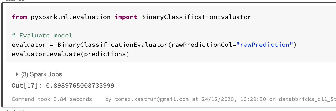
And the score of evaluated predictions is: 0.898976. What we. want to do next is to fine tune the model with the ParamGridBuilder and the CrossValidator. You can use explainParams() to see the list of parameters and the definition. Set up the ParamGrid with Regularization Parametrs, ElasticNet Parameters and number of maximum iterations.

from pyspark.ml.tuning import ParamGridBuilder, CrossValidator

# Create ParamGrid for Cross Validation
paramGrid = (ParamGridBuilder()
             .addGrid(lr.regParam, [0.01, 0.5, 2.0])
             .addGrid(lr.elasticNetParam, [0.0, 0.5, 1.0])
             .addGrid(lr.maxIter, [1, 5, 10])
             .build())

And run the cross validation.  I am taking 5-fold cross-validation. And you will see how Spark will distribute the loads among the workers using Spark Jobs. Since the matrix of ParamGrid is prepared in such way, that can be parallelised, the powerful and massive computations of Spark gives you the better and fastest compute time.

cv = CrossValidator(estimator=lr, estimatorParamMaps=paramGrid, evaluator=evaluator, numFolds=5)

# Run cross validations
cvModel = cv.fit(trainingData)

When the CV finished, check the results of model accuracy again:

# Use test set to measure the accuracy of our model on new data
predictions = cvModel.transform(testData)

# Evaluate best model
evaluator.evaluate(predictions)

The model accuracy, after cross validations, is 0.89732, which is relatively the same as before CV. So the model was stable and accurate from the beginning and CV only confirmed it.

You can also display the dataset:

selected = predictions.select("label", "prediction", "probability", "age", "occupation")
display(selected)

You can also change the graphs here and explore each observation in the dataset:

The advent is here And I wish you all Merry Christmas and a Happy New Year 2021.

The series will continue for couple of more days. And tomorrow we will explore Spark’s GraphX for Spark Core API.

Complete set of code and the Notebook is available at the Github repository.

Happy Coding and Stay Healthy!