I spend quite a bit of time at work trying to understand where we are in the business cycle. That analysis informs our capital market expectations, and, by extension, our asset allocation and portfolio risk controls.

For years now I have used a trusty old linear regression model, held together with bailing wire, duct tape, and love. It’s a good model. It predicted the 2020 recession and the 2008 recessions (yes, out of sample).

Even so, a couple of years ago I began experimenting with a neural net to (a) increase the amount of data I could shove at it and (b) possibly get a better model. Of course, I wouldn’t retire my old model just yet, I’d just run them along side each other.

So, here is the framework for forecasting a recession using a neural net in R.

What are We Trying to Predict, Anyway?

The first question we need to answer is what we want our output to be. Typically, markets see recessions coming 3 to 6 months before they officially hit. If I’m going to add value to a portfolio, I need to be rebalancing out of risk assets before everyone else. So, for my purposes, I’d like to have 9 to 12 months of lead time to get ahead of a recession.

Ideally, then, our model would look like this:

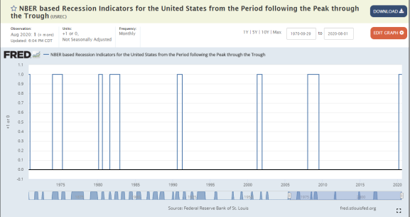
Except, instead of getting 1s concurrently with a recession, we would get them 12-months in advance. This, then, will be our output: USREC data with a 12-month lead.

The next challenge is finding the data points which reliably predict recessionary environments. Now let’s pause here for a second and acknowledge some danger…

We could data mine this thing and swap indicators in and out until we have an over-fitted model that doesn’t work going forward. Personally, I’m not a fan of that. It may be a bird-dog style analysis, pointing the way to potential information, but to me that is too dangerous. I could construct any story to “justify” random inputs to a model.

I would rather begin with indicators that (1) have been at least acknowledged and studied by others, and (2) I can build a convincing theory for how it would influence/indicate the business cycle a priori. Then I’ll plug them in and see if the model is effective.

I’d rather have an imperfect hammer than a brittle one that breaks on first impact.

Inputs

Tor the sake of this demonstration, I’ve settled on three inputs. Each of these has academic research behind it and has worked ex post. What’s more, I can build strong justifications for why each of these should both indicate and influence the economy as a whole. Of course there are others, but this is just a demonstration after all!

• Headline Unemployment
• Effective Federal Funds Rate
• The Yield Curve

Now, we won’t be using the raw figure of each of these. We are going to convert them into “signal” form. The idea is to boil-down the essence of the signal so the neural net has to do as little work as possible. That is, in my opinion, the most effective way to increase your accuracy without increasing model fragility.

The Code – Get and Wrangle Data

We are going to need five libraries for this one:

library(quantmod)
library(tidyverse)
library(nnet)
library(DALEX)
library(breakDown)

Note that DALEX and breakDown are more about visualization and understanding of the model later.

Next, let’s load our raw data. By the way, you can get these symbols from a search on the St. Louis Fed website. The symbol is immediately after the title. If you haven’t been to the FRED database… well, then we can’t be friends anymore and I can’t invite you to my birthday party.

# Get data
getSymbols( c('USREC', 'UNRATE', 'T10Y3M', 'DFF'), src = 'FRED')

# Note the differing periods of data
USREC %>% head() # Monthly data
           USREC
1854-12-01     1
1855-01-01     0
1855-02-01     0
1855-03-01     0
1855-04-01     0
1855-05-01     0

UNRATE %>% head() # Monthly data
           UNRATE
1948-01-01    3.4
1948-02-01    3.8
1948-03-01    4.0
1948-04-01    3.9
1948-05-01    3.5
1948-06-01    3.6

DFF %>% head() # Daily data
            DFF
1954-07-01 1.13
1954-07-02 1.25
1954-07-03 1.25
1954-07-04 1.25
1954-07-05 0.88
1954-07-06 0.25

T10Y3M %>% head() # Daily data (sort of)
           T10Y3M
1982-01-04   2.32
1982-01-05   2.24
1982-01-06   2.43
1982-01-07   2.46
1982-01-08   2.50
1982-01-11   2.32

Our data is not aligned, so we have a touch of work to do to wrangle it, then signal-fy it. Though the other data starts much earlier, the yield curve data doesn’t start until 1982, so we’ll cut everything before then.

# Wrangle Data, Convert to Signals
# Get all data into monthly format, starting in 1982
recessions <- USREC
unemployment <- UNRATE
fedfunds <- to.monthly(DFF)$DFF.Open
yieldcurve <- to.monthly(T10Y3M)$T10Y3M.Open

Again, I won’t cover all of the theory behind the signalification of our data, but just know that this isn’t me making random stuff up. (You should never trust anyone who says that, by the way.)

The other important component of these signals is how they are shifting through time. Because the nnet package doesn’t look backward at the data, it only takes in this moment, we need to add inputs that look backward. I’m doing that by lagging each signal by 3 months and 6 months.

# Unemployment signal: 12-month slow moving average minus
# the headline unemployment rate.
signal_unemployment <- SMA(unemployment, n = 12) - unemployment 
signal_unemployment_lag3 <- lag(signal_unemployment, n = 3)
signal_unemployment_lag6 <- lag(signal_unemployment, n = 6)

# FedFunds signal: effective federal funds rate minus the 
# maximum fedfunds rate over the past 12 months
signal_fedfunds <- fedfunds - rollmax(fedfunds, k = 12, align = 'right')
signal_fedfunds_lag3 <- lag(signal_fedfunds, n = 3)
signal_fedfunds_lag6 <- lag(signal_fedfunds, n = 6)

# Yield curve signal: 10-year US treasury yield minus the 3-month
# US treasury yield.
signal_yieldcurve <- yieldcurve
signal_yieldcurve_lag3 <- lag(signal_yieldcurve, n = 3)
signal_yieldcurve_lag6 <- lag(signal_yieldcurve, n = 6)

Recall that we want a 12-month lead time on our recession indicator, so we are going to adjust USREC data by 12-months for the purposes of training our model.

# Since we want to know if a recession is starting in the next 12 months, 
# need to lag USREC by NEGATIVE 12 months = lead(12)
signal_recessions <- recessions %>% 
  coredata() %>% # Extract core data
  lead(12) %>% # Move it 12 months earlier
  as.xts(., order.by = index(recessions)) # Reorder as an xts, with Recessions adjusted

If you remember from neural net training 101, a neural net has hyperparameters, i.e. how big the net is and how we manage weight decay. This means we can’t simply train a neural net. We have to tune it also.

Which brings us to the really sucky part: we need to divide our data into a train set, tune set, and out-of-sample test set. This means tedious “window” work. Ugh.

# Seperate data into train, test, and out-of-sample
# Training data will be through Dec 1998
# Testing data will be Jan 1999 through Dec 2012
# Out of sample will be Jan 2013 through July 2020
start_train <- as.Date('1982-08-01')
end_train <- as.Date('1998-12-31')
start_test <- as.Date('1999-01-01')
end_test <- as.Date('2012-12-31')
start_oos <- as.Date('2013-01-01')
end_oos <- as.Date('2020-07-31')
train_data <- data.frame( 'unemployment' = window( signal_unemployment,
                                                   start = start_train,
                                                   end = end_train ),
                          
                          'unemployment_lag3' = window( signal_unemployment_lag3,
                                                        start = start_train,
                                                        end = end_train ),
                          
                          'unemployment_lag6' = window( signal_unemployment_lag6,
                                                        start = start_train,
                                                        end = end_train ),
                          
                          'fedfunds' = window( signal_fedfunds,
                                               start = start_train,
                                               end = end_train),
                          
                          'fedfunds_lag3' = window( signal_fedfunds_lag3,
                                                    start = start_train,
                                                    end = end_train),
                          
                          'fedfunds_lag6' = window( signal_fedfunds_lag6,
                                                    start = start_train,
                                                    end = end_train),
                          
                          'yieldcurve' = window( signal_yieldcurve,
                                                 start = start_train,
                                                 end = end_train),
                          
                          'yieldcurve_lag3' = window( signal_yieldcurve_lag3,
                                                      start = start_train,
                                                      end = end_train),
                          
                          'yieldcurve_lag6' = window( signal_yieldcurve_lag6,
                                                      start = start_train,
                                                      end = end_train),
                          
                          'recessions' = window( signal_recessions,
                                                 start = start_train,
                                                 end = end_train) )
test_data <- data.frame( 'unemployment' = window( signal_unemployment,
                                                  start = start_test,
                                                  end = end_test ),
                         
                         'unemployment_lag3' = window( signal_unemployment_lag3,
                                                       start = start_test,
                                                       end = end_test ),
                         
                         'unemployment_lag6' = window( signal_unemployment_lag6,
                                                       start = start_test,
                                                       end = end_test ),
                         
                         'fedfunds' = window( signal_fedfunds,
                                              start = start_test,
                                              end = end_test),
                         
                         'fedfunds_lag3' = window( signal_fedfunds_lag3,
                                                   start = start_test,
                                                   end = end_test),
                         
                         'fedfunds_lag6' = window( signal_fedfunds_lag6,
                                                   start = start_test,
                                                   end = end_test),
                         
                         'yieldcurve' = window( signal_yieldcurve,
                                                start = start_test,
                                                end = end_test),
                         
                         'yieldcurve_lag3' = window( signal_yieldcurve_lag3,
                                                     start = start_test,
                                                     end = end_test),
                         
                         'yieldcurve_lag6' = window( signal_yieldcurve_lag6,
                                                     start = start_test,
                                                     end = end_test),
                         
                         'recessions' = window( signal_recessions,
                                                start = start_test,
                                                end = end_test) )
oos_data <- data.frame( 'unemployment' = window( signal_unemployment,
                                                 start = start_oos,
                                                 end = end_oos ),
                        
                        'unemployment_lag3' = window( signal_unemployment_lag3,
                                                      start = start_oos,
                                                      end = end_oos ),
                        
                        'unemployment_lag6' = window( signal_unemployment_lag6,
                                                      start = start_oos,
                                                      end = end_oos ),
                        
                        'fedfunds' = window( signal_fedfunds,
                                             start = start_oos,
                                             end = end_oos),
                        
                        'fedfunds_lag3' = window( signal_fedfunds_lag3,
                                                  start = start_oos,
                                                  end = end_oos),
                        
                        'fedfunds_lag6' = window( signal_fedfunds_lag6,
                                                  start = start_oos,
                                                  end = end_oos),
                        
                        'yieldcurve' = window( signal_yieldcurve,
                                               start = start_oos,
                                               end = end_oos),
                        
                        'yieldcurve_lag3' = window( signal_yieldcurve_lag3,
                                                    start = start_oos,
                                                    end = end_oos),
                        
                        'yieldcurve_lag6' = window( signal_yieldcurve_lag6,
                                                    start = start_oos,
                                                    end = end_oos),
                        
                        'recessions' = window( signal_recessions,
                                               start = start_oos,
                                               end = end_oos) )
colnames(train_data) <- colnames(test_data) <- colnames(oos_data) <- c( 'unemployment',
                                                                        'unemployment_lag3',
                                                                        'unemployment_lag6',
                                                                        'fedfunds',
                                                                        'fedfunds_lag3',
                                                                        'fedfunds_lag6',
                                                                        'yieldcurve',
                                                                        'yieldcurve_lag3',
                                                                        'yieldcurve_lag6',
                                                                        'recessions' )

Comment below if you have a more efficient way of doing this!

The Code – Train & Tune Our Neural Net

From here we need to make some educated, but mostly guess-like, decisions.

We must specify a minimum and maximum neural net size. I remember reading once that a neural network hidden layer should be no less than about 35% the number of inputs, and no larger than 1.5 times the total number of inputs. I’m open to critique here, but that’s what I’ll specify for the minimum and maximum.

# Hyperparameters for tuning
# Minimum net size
size_min <- (ncol(train_data) * 0.35) %>% round(0)
# Maximum net size
size_max <- (ncol(train_data) * 1.5) %>% round(0)
size <- seq(size_min, size_max, 1)

The next hyperparameter is weight decay. As far as I know, there is really no rule of thumb for this, other than it should be 0 < w < 1. For illustration, I’m going to sequence it between 0.1 and 1.5.

# Weight decay settings, start at seq(2, 50, 2) then up it.
# This figure will get divided by 100 in the coming code.
w_decay <- seq(10, 150, 2)

Yay! Now the fun part begins!

We want the neural network that delivers the best possible Brier score, and we want to output the optimal model and hyperparameters for inspection and use later. Normally I wouldn’t log the Brier scores as they go, but I want to see how net size and various weight decays effect our model, just for fun.

best_brier <- 1 # Prime variable
net_size_optimal <- 5 # Prime variable
w_decay_optimal <- 0.2 # Prime variable
# Log evolution of RMSE, rows are net size, columns are weight decay
brier_evolution <- 0
i <-  1
j <-  1
for(n in size){
  for(w in w_decay){
    
    # Train model
    model_fit <- nnet( as.matrix(train_data$recessions) ~
                         unemployment + unemployment_lag3 + unemployment_lag6 +
                         fedfunds + fedfunds_lag3 + fedfunds_lag6 +
                         yieldcurve + yieldcurve_lag3 + yieldcurve_lag6,
                       data = as.matrix(train_data),
                       maxit = 500,
                       size = n,
                       decay = w/100,
                       linout = 1 )
    
    # Test model (for hyperparameter tuning), return Brier
    model_predict <- predict( model_fit, newdata = as.matrix(test_data) )
    brier <- mean( (model_predict - test_data$recessions)^2 )
    
    # If this is the best model, store the hyperparams and the model
    if( brier < best_brier ){
      net_size_optimal <- n
      w_decay_optimal <- w/100
      best_brier <- brier
      model <- model_fit
    }
    brier_evolution[i] <- brier
    i <- i + 1
  }
}

And BOOM! We’ve got ourselves an artificial neural network!

The Code – Results

First, let’s see how our hyperparameters affected our Brier score.

# Drop Brier score into a matrix
brier_evolution <- matrix( brier_evolution, nrow = length(w_decay), ncol = length(size), byrow = FALSE )
rownames(brier_evolution) <- w_decay/100
colnames(brier_evolution) <- size
# View Brier score results
persp( x = w_decay/100,
       y = size,
       z = brier_evolution,
       ticktype = 'detailed',
       xlab = 'Weight Decay',
       ylab = 'Net Size',
       zlab = 'Brier Score',
       shade = 0.5,
       main = 'Brier Score, Effect of Net Size and Weight Decay')

Yielding

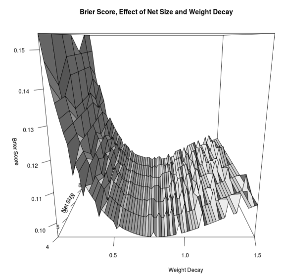
It is so interesting to me how weight decay is, by far, the most influential hyperparameter. Size matters, but not nearly as much. Also, we should note there is not too much difference between the worst model we tested and the best, as the Brier score drops from 0.15 to 0.10.

Just to put Brier scores into perspective: a score of 0 is perfect prescience, and a score of 0.50 is no better than chance. Tetlock claims that we need a Brier score of 0.30 or better to generate portfolio alpha (this is a firm-wide metric, see plot from his paper below), but it looks like 0.20 and below is really where you want to be.

At 0.10, we are on track! Of course, this is in-sample. How did we do out-of-sample?

# Use model Out of Sample, plot results
model_predict_oos <- predict( model, newdata = as.matrix(oos_data) )
data.frame( 'Date' = index( as.xts(oos_data)), 
            'Probability' = coredata(model_predict_oos) ) %>% 
  ggplot(., aes(x = Date, y = Probability) )+
  geom_line(size = 2, col = 'dodgerblue4')+
  labs(title = 'Probability of Recession in the Next 12 Months')+
  xlab('')+
  ylab('')+
  theme_light()+
  theme( axis.text = element_text(size = 12),
         plot.title = element_text(size = 18))

Which looks pretty good! Here we see that the traditional metrics produced a pretty reliable indication that 2020 would see a recession. My trusty-rusty old linear regression model predicted the same, by the way!

I am very interested to know our out-of-sample Brier score.

> brier_oos <- mean( (model_predict_oos - oos_data$recessions)^2, na.rm = T )
> brier_oos
[1] 0.04061196

0.04 is about as close to prescience as you can get. Honestly, it scares me a little because it is a bit too good. It is also suspicious to me that the model produced negative probabilities of a recession for 2014 through 2016. Before putting this into production I’d really like to know why that is.

What’s Driving These Results

Using the DALEX and breakDown packages, we can examine what is driving the results.

# Try to understand what drives the model using DALEX package
model_explanation <- explain( model, data = oos_data, predict_function = predict, y = oos_data$recessions )
bd <- break_down( model_explanation, 
                  oos_data[ length(oos_data), 1:(ncol(oos_data)-1) ], 
                  keep_distributions = T )
plot(bd)

Giving us

This illustrates the largest factors effecting the outcome in the most recent data point. It looks like the model has a standard bias of 0.081 (the intercept), and the most recent 3-month lagged yield curve data is what moved the needle most. All-in, the yield curve is the strongest signal in this data point (which doesn’t surprise me at all, it is the most well-known and widely studied because it has accurately predicted every recession since nineteensixtysomething).

We can also see how changes in any of the data points affect the output of the model

profile <- model_profile( model_explanation,
                          variables = c( 'unemployment',
                                         'unemployment_lag3',
                                         'unemployment_lag6',
                                         'fedfunds',
                                         'fedfunds_lag3',
                                         'fedfunds_lag6',
                                         'yieldcurve',
                                         'yieldcurve_lag3',
                                         'yieldcurve_lag6' ) )
plot(profile, geom = 'aggregates')

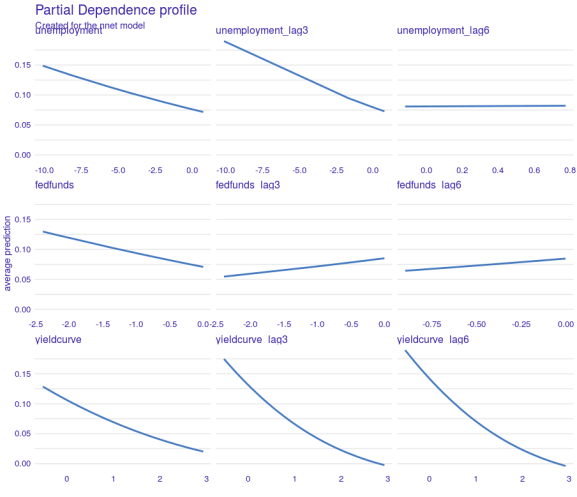
Again, the yield curve appears to be the most influential variable as changes there (x-axis) dramatically affect the output (y-axis). That said, unemployment is also a significant factor, except when lagged by 6 months. Changes there seem to have no effect.

In the end, I’d say this is a productive model. It appears robust across the various inputs, and it has an excellent out-of-sample Brier score for predicting recessions (though 2020 is our only data point for that). I am concerned that the Brier score is too good and we have created a fragile model that may not work with future inputs, and I am concerned about the negative probabilities produced in 2013 through 2016 (this may be a function of the fragility inherent in the model–those years carried unprecedented inputs).

Ultimately, there is enough here for me to dig and refine further, but I wouldn’t put this exact model into production without addressing my concerns.

As always, if you have critiques of anything here, please share them so that I can correct errors and learn!