
CPAT and the Rényi-Type Statistic; End-of-Sample Change Point Detection in R
Want to share your content on R-bloggers? click here if you have a blog, or here if you don't.
This article is also available in PDF form.
Introduction
I started my first research project as a graduate student when I was only in the MSTAT program at the University of Utah, at the very end of 2015 (or very beginning of 2016; not sure exactly when) with my current advisor, Lajos Horváth. While I am disappointed it took this long, I am glad to say that the project is finished and I am finally published.
Our article, entitled “A new class of change point test statstics of Rényi type”, is available online, published by the Journal of Business and Economic Statistics (or JBES)1 (7), but is also available on arXiv for free. In the article we present a class of statistics we call Rényi-type statistics, since they are inspired by (16). These test statistics are tailored for detecting changes that occur near the ends of the sample rather than the middle of the sample. We show that these statistics do well when structural changes happen recently (or early) in the sample, better than other popular methods.
My advisor, Lajos Horváth, and his former graduate student/assistant professor at the University of Waterloo Greg Rice developed the theory for this statistic and most of the paper had already been written when Prof. Horváth invited me to the project. I was responsible for all coding-related matters of the project, including implementing the statistics, developing and performing simulations and finding and applying the statistic to a data example. I learned a lot in the process. I was forced to learn how to organize code-intensive research projects, thus prompting (9) and (13). I learned how to write R packages and I continue to do so to organize my research projects.
This project produced CPAT, a package for change point analysis. This package exists specifically for implementing test statistics of research interest to this project but should also be useful in general. It includes not only the Rényi-type statistic but also the CUSUM statistic, the Darling-Erdös statistic, instances of the (6) statistic, and instances of the (2) statistic. To my knowledge, this is the only implementation of our new statistic and the Andrews procedure in R.
In this article I will be discussing change point testing (focusing on time series), the Rényi-type statistics, CPAT, and some examples. I will not go into full depth, including the theory of the statistic and the full simulation results; for that, see the paper we wrote. This topic was also the subject of my first Ph.D. oral defense (10), and the slides can be viewed online.
Change Point Hypothesis Testing
Suppose we have a series of data  . In change point hypothesis testing, some aspect of the distribution changes at some unknown point in time
 ![$t^* \in [T]$](https://ntguardian.files.wordpress.com/2019/07/cpatintroimg2.gif?w=578) (where
(where  ). Often we ask whether the mean is constant over the sample or not. Let
  . We wish to test

against
![\begin{displaymath} \Hypoth{A} : \mu_1=\cdots=\mu_{t^*-1}\neq \mu_{t^*}=\cdots=\mu_{T},~t^* \in [T] .\end{displaymath}](https://ntguardian.files.wordpress.com/2019/07/cpatintroimg6.gif?w=578)
Critically,  is unknown; if it were known, then we could simply use classic
  -tests known since the turn of the century. Here, though, the location of is unknown. Thus, part of the challenge is determining which of
  and
and  are true, and part of the challenge is estimating .
To some, checking for a change in  is interesting. However, change point testing extends beyond checking for changes in the mean. In fact, change point testing can attempt to detect just about any structural change in a data set. For instance, we can check for changes in the variance of a data set, or changes in a linear regression model or a time series model. There are tests for changes in functional data and even for checking for changes in distribution.
Why do people care about these things? I can easily see why an online test–where the test is attempting to detect changes as data flows in–would be interesting; I recently read of an online algorithm for detecting a change in distribution that sought to detect changes in radiation levels (a life-or-death matter in some cases) (15). However, that’s not the context I’m discussing here; I’m interested in historical changes. Why is this of interest?
First, there’s the classical example: change point testing was developed for quality control purposes. For example, a batch of widgets would be produced by a machine, and a change point test could determine if the machine ever became miscalibrated during production of the widgets. Beyond that, though, detecting a change point in a sample can be the first step to further research; the researcher would figure out why the change occurred after discovering it. There’s a third reason that every forecaster and user of time series should be aware of, though: most statistical methods using time series data require that the data be stationary, meaning that the properties of the data remain unchanging in the sample. One can hardly justify fitting a model to a data set when not all the data was produced by the same process. So change point testing checks for a particular type of pathology in data sets that everyone using time series data should watch out for.
In this article I’m not interested in estimating but only in deciding between and . Change point inference is a rich area of research and several statistics are already well known and actively used. One such statistic is the CUSUM statistic:
(  is an estimator of the long-run variance of
  ; I’ll discuss this more later.) In short, the CUSUM statistic compares subsample means of a growing window of data to the overall mean of the sample. If a subsample of the data has a mean very different from the overall mean, the null hypothesis should be rejected.
Let  be a Wiener process and
  be a Brownian bridge. If is true, then the limiting distribution of (1) is the Kolmogorov distribution as
  :
:
This is the distribution we use for hypothesis testing. Additionally, we have some power results: if is true and  for some
  , then
  . Not only that,
  may have the best power among all statistic with such .
In our paper we call such a “mid-sample” (even though in principle  could be small). We were interested more in the case where, as ,
  . We call such change points “early” or “late”. The CUSUM statistic is not as effective in those situations, but the subject of our paper was a statistic that is quite effective when the change is early or late:
Here,  is a trimming parameter such that
  but
but  . What the Rényi-type statistic does is compare the mean of the first part of the data to the mean of the rest of the data, in the latter part. If the difference between the mean of the former part of the data and the mean of the latter part becomes large in magnitude, the null hypothesis of no change should be rejected.
In our paper we showed that, whem is true, then as ,  , where
  and
and  are IID copies of
  . This establishes the distribution for computing
  -values. As for , we gave conditions on such that when is true, then
  . These conditions not only include most of those for which , (such as when ), but also conditions not covered by the CUSUM statistic in which the change tends to be early or late in the sample. For example, it’s possible to show that, as , the CUSUM statistic does not have power asymptotically when
  or when
  for
for  1$”>, but
  does when is chosen appropriately (letting
  or
or  often works).
As mentioned above, while testing for changes in the mean is nice, we want to check for structural changes not just in the mean but in for many statistics and models. And in fact we can. For example, let’s suppose we have a regression model:

Here,  is a stationary white noise process (
  and
and  has more than two moments) and
  is a sequence of stationary random vectors. We wish to test
against
![\begin{displaymath} \Hypoth{A} : \bm{\beta}_{1} = \cdots \bm{\beta}_{t^* - 1} \neq \bm{\beta}_{t^*} = \cdots = \bm{\beta}_{T},~t^* \in [T] .\end{displaymath}](https://ntguardian.files.wordpress.com/2019/07/cpatintroimg47.gif?w=578)
In fact, to do so, all you need to do is:
- Assume is true and compute an estimate
 of
of  ;
; - Compute the residuals of the model,
 ; and
; and - Compute using
![$\left\{ \hat{\epsilon}_{t} \right\}_{t \in [T]}$](https://ntguardian.files.wordpress.com/2019/07/cpatintroimg51.gif?w=578) as your data.
as your data.
This procedure does work; the statistic has the same limiting distribution under the null hypothesis as before and the test has power when the null hypothesis is false, if  and
and  also have an appropriate relationship (you can construct situations where the test does not have power, such as when
  and are orthogonal). The same procedure can be used with the CUSUM statistic, too, and both procedures have similar relationships to : the CUSUM statistic has better power when is mid-sample and the Rényi-type statistic has better power early/late sample.
This idea–use the residuals of the estimated model you’re testing for a change in–works not just for regression models but for time series models, generalized method of moments models, and I’m sure others that we haven’t considered. Later I will demonstrate checking for changes in regression models.
However, there is an issue I have ignored until now:  . This is an estimator for the long-run variance of the data. If the null hypothesis were true and there was no serial correlation in the data, one could simply use the sample variance computed on the entire sample. However, even in the uncorrelated case we use an estimator that is a consistent estimator even when the break point occurs at
 ![$t \in [T]$](https://ntguardian.files.wordpress.com/2019/07/cpatintroimg56.gif?w=578) for every . However, when working with time series data, we recommend using a kernel density estimator for the long-run variance.
for every . However, when working with time series data, we recommend using a kernel density estimator for the long-run variance.
I will not repeat the estimator here since the formula is quite involved; you can look at the original paper if you’re interested. These estimators are generally robust to heteroskedasticity (such as GARCH behavior) and autocorrelation, though they are far from perfect. In our simulations, we observed significant size inflation when there was noticeable serial correlation in the data since these estimators tend to underestimate the long-run variance. This is not a problem of the Rényi-type statistic but any statistic relying on these estimators for long-run variance estimation. Additionally, practitioners should play around with the kernel and bandwidth parameters to get the best results, since some kernels/bandwidths work better in some situations than others.
CPAT
My contribution to this project was primarily coding, from developing the implementations of these statistics to performing simulations. The result is the package CPAT (11), which is available both on CRAN and on GitHub.
While above I mentioned only the CUSUM test and the Rényi-type test, we investigated other tests as well. For instance, we considered weighted/trimmed variants of the CUSUM test, the Darling-Erdös test, the Hidalgo-Seo test, and Andrews’ test. Many of these tests are available in some form in CPAT, and have similar interfaces when sensible.
library(CPAT)


      ________ _________ _________ __________
     /       //  ___   //  ___   //         /
    /   ____//  /  /  //  /  /  //___   ___/
   /   /    /  /__/  //  /__/  /    /  /
  /   /___ /  ______//  ___   /    /  /
 /       //  /      /  /  /  /    /  /
/_______//__/      /__/  /__/    /__/        v. 0.1.0
Type citation("CPAT") for citing this R package in publications
Call me a dork, but I saw a message like this used by the package mclust (17) and Stata and I wanted to do so myself. I think it’s cool and I plan on making messages like these for my packages for no good reason (MCHT (12) has a similar on-load message).
Moving on, let’s create an artificial data set for playing with.
vec1 <- c(rnorm(100, 0), rnorm(100, 1))
Right in the middle of the sample, the mean of the data switches from 0 to 1. Thus there is a change point in the mean.
Let’s first apply the CUSUM test using the function CUSUM.test().
CUSUM.test(vec1)


        CUSUM Test for Change in Mean

data:  vec1
A = 4.0675, p-value = 8.66e-15
sample estimates:
t*
97
All of the test functions, including CUSUM.test(), produce S1-class objects of class htest, the same objects that stats statistical testing functions produce.
In this situation, the CUSUM test worked well; it rejected the null hypothesis of no change, as it should. It even made a good guess as to the location where the mean occured, estimating that  , which is close to the true location of 100. Okay, let’s try another data set.
vec2 <- as.numeric(arima.sim(200,
                             model = list(
                               order = c(1, 0, 0),
                               ar = 0.4)))
CUSUM.test(vec2)


        CUSUM Test for Change in Mean

data:  vec2
A = 1.393, p-value = 0.04127
sample estimates:
 t*
166
This data set does not have a change in mean yet the CUSUM test rejected the null hypothesis. Why is that so? This is because the default procedure for estimating the long-run variance will not work if the data is serially correlated, and in this case  with autocorrelation parameter
  . We need to switch to kernel-based long-run variance estimation.
To turn on kernel-based methods we only need to set use_kernel_var = TRUE, but there are additional choices to make. Specifically, we need to choose the kernel and the bandwidth. There are defaults but in general CPAT outsources kernel and bandwidth selection to functions from cointReg (3). Thus they use a similar interface.
The default is to use the Bartlett kernel and select the bandwidth using the method recommended by (1). We can switch to the quadratic-spectral kernel and the (14) method like so:
CUSUM.test(vec2, use_kernel_var = TRUE, kernel = "qs", bandwidth = "nw")


        CUSUM Test for Change in Mean

data:  vec2
A = 0.86106, p-value = 0.4487
sample estimates:
 t*
166
Now we get a much more reasonable -value.
Let’s work an example for detecting structural changes in linear regression models. Another package for change point detection is the package strucchange (18), and it provides a package tracking US income and expenditures. We can test for structural changes in expenditures like so:
library(strucchange)
library(dynlm)
data(USIncExp)
incexpres <- residuals(
               dynlm(d(log(expenditure)) ~ d(log(income)),
                     data = USIncExp))
CUSUM.test(incexpres, use_kernel_var = TRUE)


        CUSUM Test for Change in Mean

data:  incexpres
A = 1.5783, p-value = 0.01372
sample estimates:
 t*
320
Notice I set use_kernel_var = TRUE; there is some evidence of autocorrelation in the data, though this is a good option to turn on in general since we never know whether data is auto-correlated or not.
Okay, enough about the CUSUM statistic: let’s discuss the Rényi-type statistic. Using the Rényi-type statistic works just like using the CUSUM statistic:
HR.test(vec1)


        Horvath-Rice Test for Change in Mean

data:  vec1
D = 2.655, log(T) = 5.2983, p-value = 0.03148
sample estimates:
t*
97
The Rényi-type statistic was also able to detect the change in mean in the first sample.2 It wasn’t as authoritative as the CUSUM test but it was not incorrect. How about the second sample when we turn on the kernel-based long-run variance estimation?
HR.test(vec2, use_kernel_var = TRUE, kernel = "qs", bandwidth = "and")


        Horvath-Rice Test for Change in Mean

data:  vec2
D = 1.0009, log(T) = 5.2983, p-value = 0.8619
sample estimates:
 t*
166
The Rényi-type statistic, though, has an additional parameter to set: the trimming parameter, which above was  . Here the parameter is called
 kn, and HR.test() expects a function be supplied to it.
HR.test(vec2, use_kernel_var = TRUE, kn = sqrt)


        Horvath-Rice Test for Change in Mean

data:  vec2
D = 1.7249, sqrt(T) = 14.142, p-value = 0.3096
sample estimates:
 t*
166
We mentioned that the Rényi-type test shines when the change point occurs very early or late in the sample. Here is a demonstration:
vec3 <- c(rnorm(5, mean = 0), rnorm(195, mean = 1))
CUSUM.test(vec3)
HR.test(vec3)


        CUSUM Test for Change in Mean

data:  vec3
A = 0.803, p-value = 0.5393
sample estimates:
t*
27


        Horvath-Rice Test for Change in Mean

data:  vec3
D = 2.6722, log(T) = 5.2983, p-value = 0.02991
sample estimates:
t*
 5
Here the CUSUM statistic fails to detect the early structural change but the Rényi-type statistic does not.3In general, the CUSUM statistic will have better power when the change occurs near the middle of the sample, while the Rényi-type statistic will have better power when the change happens early or late.
Let’s wrap up our introduction to HR.test() with a demonstration of testing for changes in regression models:
HR.test(incexpres, use_kernel_var = TRUE)


        Horvath-Rice Test for Change in Mean

data:  incexpres
D = 1.4198, log(T) = 6.2246, p-value = 0.5257
sample estimates:
t*
24
Finally, let’s consider some other statistics available in CPAT. First, there’s the Darling-Erdös statistic. Let

When  , this is known as the weighted CUSUM statistic, and in general, for
  \frac{1}{2}$"> we know this as the weighted and trimmed CUSUM statistic.4 This version of the CUSUM statistic should handle early/late change points better, though our (unreported) simulations suggest that the Rényi-type statistic has better power in the extreme cases we considered. The Darling-Erdös statistic is

where  . It exists in CPAT as
 DE.test().
DE.test(vec1)
DE.test(vec2, use_kernel_var = TRUE, kernel = "qs", bandwidth = "nw")
DE.test(vec3)


        Darling-Erdos Test for Change in Mean

data:  vec1
A = 6.9468, a(log(T)) = 1.8261, b(log(T)) = 3.0180, p-value = 0.001922
sample estimates:
t*
97


        Darling-Erdos Test for Change in Mean

data:  vec2
A = 1.1004, a(log(T)) = 1.8261, b(log(T)) = 3.0180, p-value = 0.486
sample estimates:
 t*
166


        Darling-Erdos Test for Change in Mean

data:  vec3
A = 1.4832, a(log(T)) = 1.8261, b(log(T)) = 3.0180, p-value = 0.3648
sample estimates:
t*
 5


DE.test(incexpres, use_kernel_var = TRUE)


        Darling-Erdos Test for Change in Mean

data:  incexpres
A = 1.8017, a(log(T)) = 1.9123, b(log(T)) = 3.3864, p-value = 0.2811
sample estimates:
 t*
320
Then there’s the Hidalgo-Seo statistic, existing in CPAT as HS.test(). This function was designed for working with univariate data; one could try to use HS.test() for testing for changes in regression models as we did above, but that would not be using the same statistic that Hidalgo and Seo presented.5 Additionally, this function does not have the same interface as the others in CPAT; it does not use kernel-based methods for long-run variance estimation but uses the procedure presented in the paper where the residuals are allowed to follow an  process. Thus, there is a parameter,
 corr, for controlling whether this approach is used or not (if not, the residuals are treated as if they are IID); corr = FALSE by default.
HS.test(vec1)
HS.test(vec2, corr = TRUE)
HS.test(vec3)


        Hidalgo-Seo Test for Change in Mean

data:  vec1
A = 10.638, Correlated Residuals = TRUE, p-value = 0.009749
sample estimates:
t*
97


        Hidalgo-Seo Test for Change in Mean

data:  vec2
A = 2.0908, Correlated Residuals = TRUE, p-value = 0.505
sample estimates:
 t*
166


        Hidalgo-Seo Test for Change in Mean

data:  vec3
A = 5.7549, Correlated Residuals = TRUE, p-value = 0.1065
sample estimates:
t*
 5
Finally, there’s Andrews’ test. This is the most distinct test of the ones presented here. The version implemented here is designed for detecting late changes in the sample only; there is not a version for early or mid-sample changes. Apparently at least one person uses this test, which was surprising to me; I thought it would be the least used. But since someone is using the test, I may need to implement these other versions of Andrews’ test; I give the people what they want!
Andrews’ test does not test the same set of hypotheses we considered above; instead, the version for late changes claims, under the null hypothesis, that the change happens after some point  in the sample, and that
  is known (but supposedly is not); in short, under ,
  . We consider this an odd setup; if this were true and we knew where the change might happen, we could simply use a two-sample -test (or the equivalent for, say, regression models) like students learn in statistics 101 classes and the resulting test would be, provably, the most powerful test.
Nevertheless, CPAT supports this test via the Andrews.test() function. Different versions of the test will be used depending on the input. If the data is univariate, the version run will be specifically made for univariate data. Andrews.test() requires that the parameter  be set, since this is a necessary input for the alternative hypothesis that cannot be guessed; this is the first point in the sample where a change could occur.
Andrews.test(vec1, 100)


        Andrews' Test for Structural Change

data:  vec1
S = 96.49, m = 100, p-value = 1
Andrews’ procedure does not worry about long-run variance estimation like the other statistics; this is because of the data-dependent subsampling procedure Andrews’ test uses for computing -values. (The setup of the test may be silly, but the end result is fascinating!)
Andrews.test(vec2, 100)


        Andrews' Test for Structural Change

data:  vec2
S = 100.92, m = 100, p-value = 1
Andrews’ test was designed for detecting changes near the ends of the sample. In this last example, the change occurs in the last 5 observations, and I tell the test that the change will happen after observation 190.
Andrews.test(rev(vec3), 190)


        Andrews' Test for Structural Change

data:  rev(vec3)
S = 13.253, m = 10, p-value = 0.6188
Again, the Rényi-type statistic comes out on top.
I mentioned that different versions of Andrews’ test will be used depending on the input. If the input to the test is a data.frame, then Andrews.test() will expect the user to supply a formula; it’s expecting to test for a structural change in a regression model.
mod <- dynlm(d(log(expenditure)) ~ d(log(income)), data = USIncExp)
X <- as.data.frame(model.frame(mod))
names(X) <- c("exp", "inc")
Andrews.test(exp ~ inc, x = X, M = 300)


        Andrews' Test for Structural Change

data:  X
S = 1.7764, m = 205, p-value = 0.9792
Change Point Detection Example: Beta
Now that I’ve shown how to use the main functions of CPAT, I want to demonstrate detecting structural change in a real-world context. There is an example in the paper that demonstrates that the Rényi-type statistic could have detected changes in the (5) five-factor model when estimated for a portfolio of banking stocks around the time of the 2008 financial crisis. Additionally, the functions presented here would have detected a change in the relationship between US worker productivity and compensation, which I wrote about before (8).
Let’s look at a different example; beta. Consider a stock; let  be the return of this stock at time . Let
  be the risk-free rate of return (such as the return from US Treasury notes) and let
  be the market return (perhaps the return from investing in an S&P 500 index fund) at time . If you’re familiar with finance, you may have heard of quantities such as alpha and beta. Alpha is the excess return of the stock over the market; that is, how much of a profit one gets for investing in the stock rather than the market (less the risk-free rate of return). Beta, on the other hand, measures how much the stock moves like the market. If a stock’s beta is zero, it has no relation with the market; if its beta is positive, the stock does well when the market does well on average; and if beta is negative, the stock does well when the market does poorly, on average. If the beta is above one, the stock is more sensitive to the market (so a beta of two suggests that if the market had a return 1% in excess of average, the stock should be 2% in excess of its own average), while a beta less than one suggests a stock less sensitive to the movements of the market (an analogous statement can be made for betas above or below negative one).
I remember learning about beta in my mathematical finance class and a student asking “Why should beta be constant over time?” That’s a great observation, and one that I’m here to address. See, alpha and beta are computed by estimating parameter  and
and  (for alpha and beta, respectively) in the regression model

Thus, checking that alpha and beta are constant over time equates to performing a change point hypothesis test. When estimating , it makes sense for people practicing quantitative finance to check for change points. If there is a change point (or perhaps more than one), then using more data won’t make the estimate of better, since some of the data was data produced by a different than the most recent one.
CPAT comes with a subset of the Fama-French factors needed for estimating Fama-French five-factor models. We will use only some of those factors here to compute the that most investors are familiar with. Since the data set also comes with estimates of the risk-free rate of return, we will use those as well.
Now for the stock. Let’s study Valeant Pharmaceuticals (now known as Bausch Health, in an effort to escape the reputation they rightfully earned), the subject of an episode of Dirty Money (4). Valeant had ticker symbol VRX (now BHC) and after 2008 it had a meteoric rise until Valeant’s business practices of buying drugs and hiking their prices to absurd, unaffordable levels–along with outright fraudulent behavior–attracted unwanted attention, preceding the collapse of the stock.
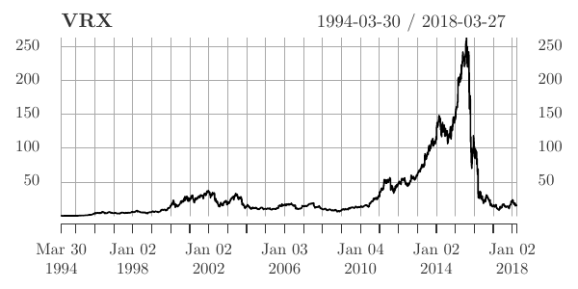
We can download the data for VRX from Quandl.
library(Quandl)
library(xts)

VRX <- Quandl("WIKI/VRX", type = "xts")
VRX <- VRX$`Adj. Close`
names(VRX) <- "VRX"
The Fama-French factors are stored in the data.frame ff. Let’s next create an object containing both VRX’s log returns and the Fama-French factors.
data(ff)
ff <- as.xts(ff, order.by = as.Date(rownames(ff), "%Y%m%d"))
VRX <- diff(log(VRX)) * 100

VRXff <- merge(VRX, ff, all = FALSE)[-1,]
Let’s now compute the alpha and beta of VRX and test for structural change. Note that RF is the risk-free rate of return and Mkt.RF is the market return less the risk-free rate.
mod <- dynlm(I(VRX - RF) ~ Mkt.RF, data = as.zoo(VRXff["2009/"]))
CUSUM.test(residuals(mod), use_kernel_var = TRUE)


        CUSUM Test for Change in Mean

data:  residuals(mod)
A = 1.9245, p-value = 0.001214
sample estimates:
  t*
1659
The CUSUM test does detect a change. Additionally, it believes the change happened in August 2015. This date is a good guess; the first bad news for Valeant occurred in October 2015, when a short seller named Andrew Left claimed that Valeant was engaging in perhaps illegal relations with a pharmacist named Philidor Rx Services.
But that conclusion comes after having 2016 and 2017 data, when Valeant had clearly fallen from their “prime.” What if it was the end of 2015 and you were recalibrating your models then? Would you have detected a change from the CUSUM test? Or even the Darling-Erdös test?
Let’s find out.
mod2 <- dynlm(I(VRX - RF) ~ Mkt.RF, data = as.zoo(VRXff["2009/2015"]))
CUSUM.test(residuals(mod2), use_kernel_var = TRUE)
DE.test(residuals(mod2), use_kernel_var = TRUE)


        CUSUM Test for Change in Mean

data:  residuals(mod2)
A = 0.96233, p-value = 0.3126
sample estimates:
  t*
1652


        Darling-Erdos Test for Change in Mean

data:  residuals(mod2)
A = 2.8559, a(log(T)) = 2.0057, b(log(T)) = 3.8000, p-value = 0.1086
sample estimates:
  t*
1690
If you were just using the CUSUM test: no, you would not have noticed a change. The Darling-Erdös test is closer, but not convincing.
How about the Rényi-type test?
HR.test(residuals(mod2), use_kernel_var = TRUE, kn = sqrt)


        Horvath-Rice Test for Change in Mean

data:  residuals(mod2)
D = 3.6195, sqrt(T) = 41.976, p-value = 0.00118
sample estimates:
  t*
1690
Yes, you would have detected a change if you were using the Rényi-type statistic.
Conclusion
First: how would I expect people to use the Rényi-type statistic in practice? Well, I’m not expecting the statistic to replace other statistics, such as the CUSUM statistic. The Rényi-type statistic has strengths not well emulated by other test statistics, but it also has relative weaknesses, too. My thought is that the test should be used along with those other tests. If both tests agree, cool; if they disagree, check where the tests suggest the change occurred and decide if you believe the test that rejected. And you should usually use kernel-based long-run variance estimation methods unless you have good reason not to do so.
We are continuing to study the Rényi-type statistic and hope to get more publications from it. One issue I think we did not adequately address is how to select the trimming parameter. This is an important decision that can change the results of tests, and we don’t have any rigorous suggestions on how to pick the parameter other than and seem to work well, though one sometimes works better than the other.
We have a lot of material for those who want to learn more about this subject. There’s the aforementioned paper that goes into more depth than this brief article, and gives more convincing evidence that our new statistic works well in early/late change contexts. Additionally, the CPAT archive contains a version of the package that includes not only the version of the software used for the paper but also the code that allows others to recreate and “play” with our simulations. (In other words I attempted to make our work reproducible.)
If you’re using CPAT, I want to hear your feedback! I got feedback from one user and not only did it make my day it also gave me some idea of what I should be working on to release in future versions. And perhaps user questions will turn into future research.
Finally, if you’re working with time series data and are unaware of or not performing change point analysis, I hope that this article was a good introduction to the subject and convinced you to start using these methods. As my example demonstrated, good change point detection can matter even in a monetary way. Using more data won’t help if the old data is no longer relevant.
Bibliography
- 1
- Donald W. K. Andrews.
Heteroskedasticity and autocorrelation consistent covariance matrix estimation.
Econometrica, 59 (3): 817-858, May 1991. - 2
- Donald W. K. Andrews.
End-of-sample instability tests.
Econometrica, 71 (6): 1661-1694, 2003.
ISSN 00129682, 14680262.
URL https://www.jstor.org/stable/1555535. - 3
- Philipp Aschersleben and Martin Wagner.
cointReg: Parameter Estimation and Inference in a Cointegrating Regression, 2016.
URL https://CRAN.R-project.org/package=cointReg.
R package version 0.2.0. - 4
- Erin Lee Carr.
Dirty money; drug short.
Film, January 2018. - 5
- Eugene F. Fama and Kenneth R. French.
A five-factor asset pricing model.
Journal of Financial Economics, 116 (1): 1 – 22, 2015.
ISSN 0304-405X.
doi: rm10.1016/j.jfineco.2014.10.010.
URL http://www.sciencedirect.com/science/article/pii/S0304405X14002323. - 6
- Javier Hidalgo and Myung Hwan Seo.
Testing for structural stability in the whole sample.
Journal of Econometrics, 175 (2): 84 – 93, 2013.
ISSN 0304-4076.
doi: rm10.1016/j.jeconom.2013.02.008.
URL http://www.sciencedirect.com/science/article/pii/S0304407613000626. - 7
- Lajos Horváth, Curtis Miller, and Gregory Rice.
A new class of change point test statistics of Rényi type.
Journal of Business & Economic Statistics, 0 (0): 1-19, 2019.
doi: rm10.1080/07350015.2018.1537923.
URL https://doi.org/10.1080/07350015.2018.1537923. - 8
- Curtis Miller.
Did wages detach from productivity in 1973? an investigation.
Website, September 2016.
URL https://ntguardian.wordpress.com/2016/09/12/wages-detach-productivity-1973/.
Blog. - 9
- Curtis Miller.
How should i organize my R research projects?
Website, August 2018a.
URL https://ntguardian.wordpress.com/2018/08/02/how-should-i-organize-my-r-research-projects/.
Blog. - 10
- Curtis Miller.
Change point statistics of Rényi type.
Online, November 2018b.
URL http://rgdoi.net/10.13140/RG.2.2.36035.45604.
Presentation. - 11
- Curtis Miller.
CPAT: Change Point Analysis Tests, 2018c.
URL https://cran.r-project.org/package=CPAT.
R package version 0.1.0. - 12
- Curtis Miller.
MCHT: Bootstrap and Monte Carlo Hypothesis Testing, 2018d.
R package version 0.1.0. - 13
- Curtis Miller.
Organizing R research projects: CPAT, a case study.
Website, February 2019.
URL https://ntguardian.wordpress.com/2019/02/04/organizing-r-research-projects-cpat-case-study/.
Blog. - 14
- Whitney K. Newey and Kenneth D. West.
Automatic lag selection in covariance matrix estimation.
Review of Economic Studies, 61 (4): 631-653, 1994. - 15
- Oscar Hernan Madrid Padilla, Alex Athey, Alex Reinhart, and James G. Scott.
Sequential nonparametric tests for a change in distribution: An application to detecting radiological anomalies.
Journal of the American Statistical Association, 114 (526): 514-528, 2019.
doi: rm10.1080/01621459.2018.1476245.
URL https://doi.org/10.1080/01621459.2018.1476245. - 16
- Alfréd Rényi.
On the theory of order statistics.
Acta Mathematica Academiae Scientiarum Hungarica, 4 (3): 191-231, Sep 1953.
ISSN 1588-2632.
doi: rm10.1007/BF02127580.
URL https://doi.org/10.1007/BF02127580. - 17
- Luca Scrucca, Michael Fop, Thomas Brendan Murphy, and Adrian E. Raftery.
mclust 5: clustering, classification and density estimation using Gaussian finite mixture models.
The R Journal, 8 (1): 205-233, 2016.
URL https://journal.r-project.org/archive/2016-1/scrucca-fop-murphy-etal.pdf. - 18
- Achim Zeileis, Christian Kleiber, Walter Krämer, and Kurt Hornik.
Testing and dating of structural changes in practice.
Computational Statistics & Data Analysis, 44: 109-123, 2003.
About this document …
CPAT and the Rényi-type Statistic: End-of-Sample Change Point Detection in R
This document was generated using the LaTeX2HTML translator Version 2019 (Released January 1, 2019)
The command line arguments were:
latex2html -split 0 -nonavigation -lcase_tags -image_type gif simpledoc.tex
The translation was initiated on 2019-07-23
Footnotes
- …JBES)1
- It has yet to appear in the print edition.
- … sample.2
HR.test()also supplies an estimate for when the change occurred, but unlike for the CUSUM statistic there isn’t theory to back it up and we don’t recommend using it over the CUSUM estimate. It’s the location where the difference in the sub-sample means is greatest. In later versions we may delete this feature.- … not.3
- Astute readers may notice that
 . We don’t need
  or
or  in order for a change to be detected; in fact, in our simulations this was often not the case, yet the Rényi-type statistic could still detect such early changes.
 - … statistic.4
- There isn’t a publicly available implementation of the weighted-trimmed CUSUM statistic in CPAT, though we may add this in the future, especially if users request it.
- … presented.5
- A statistic designed specifically for linear regression models may be coming in the future.
Packt Publishing published a book for me entitled Hands-On Data Analysis with NumPy and Pandas, a book based on my video course Unpacking NumPy and Pandas. This book covers the basics of setting up a Python environment for data analysis with Anaconda, using Jupyter notebooks, and using NumPy and pandas. If you are starting out using Python for data analysis or know someone who is, please consider buying my book or at least spreading the word about it. You can buy the book directly or purchase a subscription to Mapt and read it there.
If you like my blog and would like to support it, spread the word (if not get a copy yourself)!
R-bloggers.com offers daily e-mail updates about R news and tutorials about learning R and many other topics. Click here if you're looking to post or find an R/data-science job.
Want to share your content on R-bloggers? click here if you have a blog, or here if you don't.