
Markov chain Monte Carlo doesn’t “explore the posterior”
Want to share your content on R-bloggers? click here if you have a blog, or here if you don't.
First some background, then the bad news, and finally the good news.
Spoiler alert: The bad news is that exploring the posterior is intractable; the good news is that we don’t need to explore all of it.
Sampling to characterize the posterior
There’s a misconception among Markov chain Monte Carlo (MCMC) practitioners that the purpose of sampling is to explore the posterior. For example, I’m writing up some reproducible notes on probability theory and statistics through sampling (in pseudocode with R implementations) and have just come to the point where I’ve introduced and implemented Metropolis and want to use it to exemplify convergence mmonitoring. So I did what any right-thinking student would do and borrowed one of my mentor’s diagrams (which is why this will look familiar if you’ve read the convergence monitoring section of Bayesian Data Analysis 3).
First M steps of of isotropic random-walk Metropolis with proposal scale normal(0, 0.2) targeting a bivariate normal with unit variance and 0.9 corelation. After 50 iterations, we haven’t found the typical set, but after 500 iterations we have. Then after 5000 iterations, everything seems to have mixed nicely through this two-dimensional example.
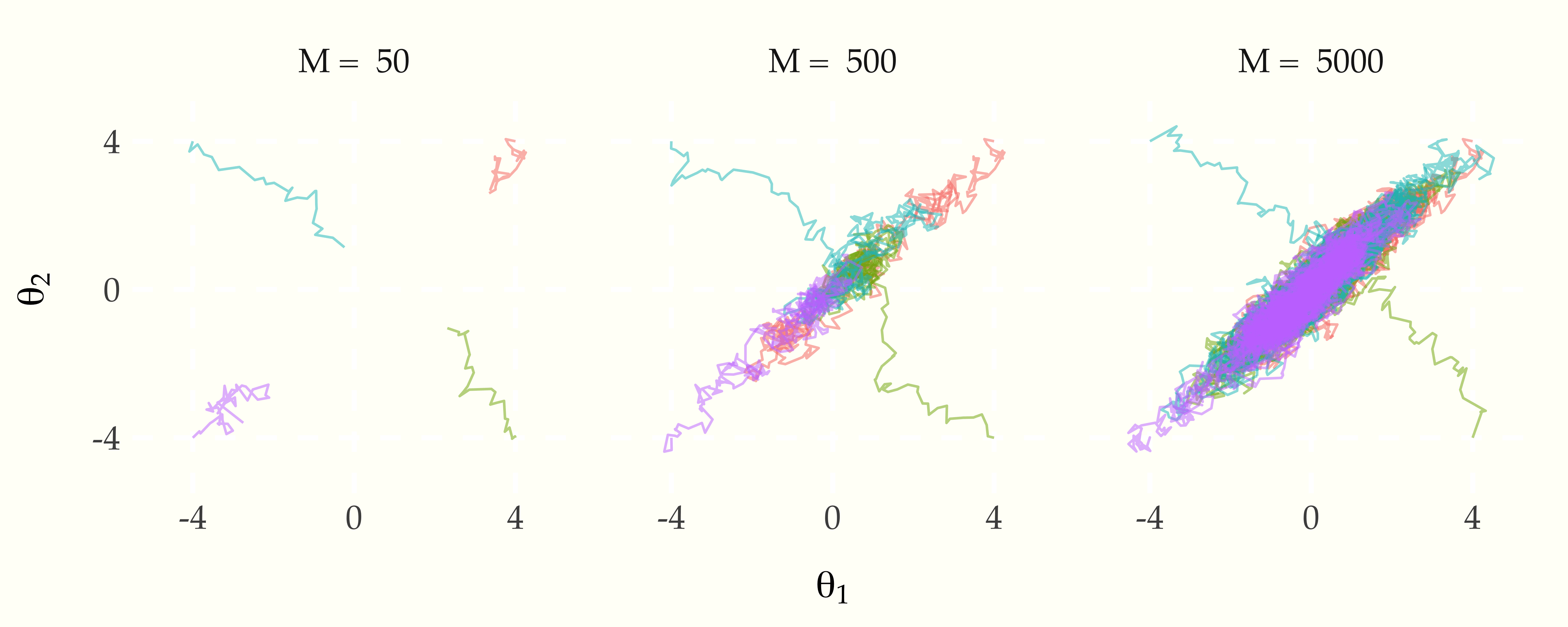
This two-dimensional traceplot gives the misleading impression that the goal is to make sure each chain has moved through the posterior. This low-dimensional thinking is nothing but a trap in higher dimensions. Don’t fall for it!
Bad news from higher dimensions
It’s simply intractable to “cover the posterior” in high dimensions. Consider a 20-dimensional standard normal distribution. There are 20 variables, each of which may be positive or negative, leading to a total of 
Good news in expectation
Bayesian inference is based on probability, which means integrating over the posterior density. This boils down to computing expectations of functions of parameters conditioned on data. This we can do.
For example, we can construct point estimates that minimize expected square error by using posterior means, which are just expectations conditioned on data, which are in turn integrals, which can be estimated via MCMC,
![\begin{array}{rcl} \hat{\theta} & = & \mathbb{E}[\theta \mid y] \\[8pt] & = & \int_{\Theta} \theta \times p(\theta \mid y) \, \mbox{d}\theta. \\[8pt] & \approx & \frac{1}{M} \sum_{m=1}^M \theta^{(m)},\end{array}](http://s0.wp.com/latex.php?latex=%5Cbegin%7Barray%7D%7Brcl%7D+%5Chat%7B%5Ctheta%7D+%26+%3D+%26+%5Cmathbb%7BE%7D%5B%5Ctheta+%5Cmid+y%5D+%5C%5C%5B8pt%5D+%26+%3D+%26+%5Cint_%7B%5CTheta%7D+%5Ctheta+%5Ctimes+p%28%5Ctheta+%5Cmid+y%29+%5C%2C+%5Cmbox%7Bd%7D%5Ctheta.+%5C%5C%5B8pt%5D+%26+%5Capprox+%26+%5Cfrac%7B1%7D%7BM%7D+%5Csum_%7Bm%3D1%7D%5EM+%5Ctheta%5E%7B%28m%29%7D%2C%5Cend%7Barray%7D&bg=ffffff&%23038;fg=000000&%23038;s=0 "\begin{array}{rcl} \hat{\theta} & = & \mathbb{E}[\theta \mid y] \\[8pt] & = & \int_{\Theta} \theta \times p(\theta \mid y) \, \mbox{d}\theta. \\[8pt] & \approx & \frac{1}{M} \sum_{m=1}^M \theta^{(m)},\end{array}")
where }, \ldots, \theta^{(M)}")
.")
If we want to calculate predictions, we do so by using sampling to calculate the integral required for the expectation,
![p(\tilde{y} \mid y) \ = \ \mathbb{E}[p(\tilde{y} \mid \theta) \mid y] \ \approx \ \frac{1}{M} \sum_{m=1}^M p(\tilde{y} \mid \theta^{(m)}),](http://s0.wp.com/latex.php?latex=p%28%5Ctilde%7By%7D+%5Cmid+y%29+%5C+%3D+%5C+%5Cmathbb%7BE%7D%5Bp%28%5Ctilde%7By%7D+%5Cmid+%5Ctheta%29+%5Cmid+y%5D+%5C+%5Capprox+%5C+%5Cfrac%7B1%7D%7BM%7D+%5Csum_%7Bm%3D1%7D%5EM+p%28%5Ctilde%7By%7D+%5Cmid+%5Ctheta%5E%7B%28m%29%7D%29%2C&bg=ffffff&%23038;fg=000000&%23038;s=0 "p(\tilde{y} \mid y) \ = \ \mathbb{E}[p(\tilde{y} \mid \theta) \mid y] \ \approx \ \frac{1}{M} \sum_{m=1}^M p(\tilde{y} \mid \theta^{(m)}),")
If we want to calculate event probabilities, it’s just the expectation of an indicator function, which we can calculate through sampling, e.g.,
