
Creating landscapes and simulating species occupation with MetaLandSim
Want to share your content on R-bloggers? click here if you have a blog, or here if you don't.
MetaLandSim is an R package I’ve developed to simulate metapopulational dynamics on an habitat network. It also computes a lot of landscape connectivity metrics and simulates range expansion (check the manual if you are interested).
I’ve mentioned it here frequently, and sometimes I like to post a simple script that I used to answer a user’s question, or a that I’ve written for any other reason. This is a run through the main functions of the package.
Much more complex uses are possible, and I’ve already published a paper with some advanced uses of the package (with another one on the way – I hope!).
Let’s start!
First of all, as always, we should load the package:
# load the package
library(MetaLandSim)
## Warning: package 'MetaLandSim' was built under R version 3.5.1
## Loading required package: tcltk
## Loading required package: igraph
## Warning: package 'igraph' was built under R version 3.5.1
## ## Attaching package: 'igraph'
## The following objects are masked from 'package:stats':
##
##     decompose, spectrum
## The following object is masked from 'package:base':
##
##     union
Now, to create a random landscape of 10 patches with mean area of 0.2 hectares, and with the landscape mosaic being a square with 1000 meters side.
The species mean dispersal ability is 120 meters (this is merely for graphical purposes, in order to connect the patches producing the graph).
A plot with the landscape graph is displayed graphically.
So… let’s create the landscape:
# set up the plotting window
plot.new()
par(mfrow = c(1,2))

set.seed(200)
rl1 <- rland.graph(mapsize = 1000,
                   dist_m = 80,
                   areaM = 0.2,
                   areaSD = 0.115,
                   Npatch = 10,
                   disp = 120,
                   plotG = TRUE)

# look at the node.characteristics
nodes <- rl1$nodes.characteristics
nodes
And this data frame shows the characteristics of each patch:
##           x         y      areas    radius cluster    colour nneighbour ID
## 1  533.7724 583.76503 0.18420882 24.214766       1 #FF0000FF   102.9282  1
## 2  454.3649 649.25291 0.10651184 18.412977       1 #FF0000FF   102.9282  2
## 3  589.5783 691.03989 0.04015217 11.305234       2 #FFBF00FF   120.9222  3
## 4  667.3315 839.29374 0.08311528 16.265428       3 #80FF00FF   167.4060  4
## 5  711.6001  96.50122 0.36824823 34.236976       4 #00FF40FF   149.0693  5
## 6  523.8247 235.35054 0.12806475 20.190165       5 #00FFFFFF   112.1129  6
## 7  566.7674 131.78785 0.01301267  6.435886       5 #00FFFFFF   112.1129  7
## 8  153.7271 649.28867 0.28659388 30.203587       6 #0040FFFF   300.6378  8
## 9  383.2137 307.29806 0.15232900 22.019951       7 #8000FFFF   157.9491  9
## 10 922.1776 646.32962 0.20853287 25.763943       8 #FF00BFFF   319.6587 10
# label the node points
text(x = nodes[,'x'],y = nodes[,'y'], pos = 2, offset = .5, labels = as.character(nodes[,'ID']))

# look at information associated with this object
# note the class is a landscape
class(rl1)
## [1] "landscape"
names(rl1)
## [1] "mapsize"               "minimum.distance"      "mean.area"
## [4] "SD.area"               "number.patches"        "dispersal"
## [7] "nodes.characteristics"
In order to look at the structure of the object ‘rl1’, our random landscape (the graph):
str(rl1)
## List of 7
##  $ mapsize              : num 1000
##  $ minimum.distance     : num 80
##  $ mean.area            : num 0.157
##  $ SD.area              : num 0.11
##  $ number.patches       : int 10
##  $ dispersal            : num 120
##  $ nodes.characteristics:'data.frame':   10 obs. of  8 variables:
##   ..$ x         : num [1:10] 534 454 590 667 712 ...
##   ..$ y         : num [1:10] 583.8 649.3 691 839.3 96.5 ...
##   ..$ areas     : num [1:10] 0.1842 0.1065 0.0402 0.0831 0.3682 ...
##   ..$ radius    : num [1:10] 24.2 18.4 11.3 16.3 34.2 ...
##   ..$ cluster   : int [1:10] 1 1 2 3 4 5 5 6 7 8
##   ..$ colour    : Factor w/ 8 levels "#0040FFFF","#00FF40FF",..: 6 6 8 5 2 3 3 1 4 7
##   ..$ nneighbour: num [1:10] 103 103 121 167 149 ...
##   ..$ ID        : int [1:10] 1 2 3 4 5 6 7 8 9 10
##  - attr(*, "class")= chr "landscape"
Obtaining the summary of the landscape:
summary_landscape(rl1)
##                                             Value
## landscape area (hectares)                 100.000
## number of patches                          10.000
## mean patch area (hectares)                  0.157
## SD patch area                               0.110
## mean distance amongst patches (meters)    391.228
## minimum distance amongst patches (meters)  60.300
This landscape is really a mathematical graph, where edges connect nodes (points) if they are within the dispersal distance:
help('edge.graph')
e1 <- edge.graph(rl1)
e1
##   ID node A node B   area ndA  area ndB       XA       YA       XB
## 1  1      2      1 0.10651184 0.1842088 454.3649 649.2529 533.7724
## 2  2      7      6 0.01301267 0.1280648 566.7674 131.7879 523.8247
##         YB distance
## 1 583.7650 102.9282
## 2 235.3505 112.1129
And now, let’s populate the patches with a species, considering that red is empty, green is occupied:
help('species.graph')
set.seed(10)
sp_t0 <- species.graph(rl = rl1,
                       method = "percentage",
                       parm = 50,
                       nsew = "none",
                       plotG = TRUE)

# label the node points
text(x = nodes[,'x'],y = nodes[,'y'], pos = 2, offset = 0.5, labels = as.character(nodes[,'ID']))
This figure shows the empty landscape on the left (rl1) and the occupied on the right (sp_t0):

Look at the information regarding this object. Note the class is metapopulation also note the addition of element ‘distance.to.neighbors’.
Let’s check the class of object ‘sp_t0’:
class(sp_t0)
## [1] "metapopulation"
names(sp_t0)
## [1] "mapsize"                "minimum.distance"
## [3] "mean.area"              "SD.area"
## [5] "number.patches"         "dispersal"
## [7] "distance.to.neighbours" "nodes.characteristics"
And now, looking at the structure of ‘sp_t0’:
str(sp_t0)
## List of 8
##  $ mapsize               : num 1000
##  $ minimum.distance      : num 80
##  $ mean.area             : num 0.157
##  $ SD.area               : num 0.11
##  $ number.patches        : num 10
##  $ dispersal             : num 120
##  $ distance.to.neighbours:'data.frame':  10 obs. of  10 variables:
##   ..$ 1 : num [1:10] 0 103 121 288 519 ...
##   ..$ 2 : num [1:10] 103 0 142 285 610 ...
##   ..$ 3 : num [1:10] 121 142 0 167 607 ...
##   ..$ 4 : num [1:10] 288 285 167 0 744 ...
##   ..$ 5 : num [1:10] 519 610 607 744 0 ...
##   ..$ 6 : num [1:10] 349 420 460 621 234 ...
##   ..$ 7 : num [1:10] 453 530 560 715 149 ...
##   ..$ 8 : num [1:10] 386 301 438 548 785 ...
##   ..$ 9 : num [1:10] 315 349 436 603 390 ...
##   ..$ 10: num [1:10] 393 468 336 320 589 ...
##  $ nodes.characteristics :'data.frame':  10 obs. of  9 variables:
##   ..$ x         : num [1:10] 534 454 590 667 712 ...
##   ..$ y         : num [1:10] 583.8 649.3 691 839.3 96.5 ...
##   ..$ areas     : num [1:10] 0.1842 0.1065 0.0402 0.0831 0.3682 ...
##   ..$ radius    : num [1:10] 24.2 18.4 11.3 16.3 34.2 ...
##   ..$ cluster   : int [1:10] 1 1 2 3 4 5 5 6 7 8
##   ..$ colour    : Factor w/ 8 levels "#0040FFFF","#00FF40FF",..: 6 6 8 5 2 3 3 1 4 7
##   ..$ nneighbour: num [1:10] 103 103 121 167 149 ...
##   ..$ ID        : int [1:10] 1 2 3 4 5 6 7 8 9 10
##   ..$ species   : num [1:10] 1 0 1 1 1 1 0 0 0 0
##  - attr(*, "class")= chr "metapopulation"
Look at some elements like distance.to.neighbors:
head(sp_t0$distance.to.neighbours, n = 3)
##          1        2        3        4        5        6        7        8
## 1   0.0000 102.9282 120.9222 288.3278 518.6990 348.5565 453.1799 385.6524
## 2 102.9282   0.0000 141.5232 285.4300 609.6756 419.6902 529.5323 300.6378
## 3 120.9222 141.5232   0.0000 167.4060 606.9312 460.4089 559.7171 437.8463
##          9       10
## 1 314.8046 393.4118
## 2 349.2787 467.8218
## 3 435.7111 335.5909
Note the species column in nodes.characteristics, it contains the information on the presence and absence of the focal species in the habitat network:
sp_t0$nodes.characteristics
##           x         y      areas    radius cluster    colour nneighbour ID
## 1  533.7724 583.76503 0.18420882 24.214766       1 #FF0000FF   102.9282  1
## 2  454.3649 649.25291 0.10651184 18.412977       1 #FF0000FF   102.9282  2
## 3  589.5783 691.03989 0.04015217 11.305234       2 #FFBF00FF   120.9222  3
## 4  667.3315 839.29374 0.08311528 16.265428       3 #80FF00FF   167.4060  4
## 5  711.6001  96.50122 0.36824823 34.236976       4 #00FF40FF   149.0693  5
## 6  523.8247 235.35054 0.12806475 20.190165       5 #00FFFFFF   112.1129  6
## 7  566.7674 131.78785 0.01301267  6.435886       5 #00FFFFFF   112.1129  7
## 8  153.7271 649.28867 0.28659388 30.203587       6 #0040FFFF   300.6378  8
## 9  383.2137 307.29806 0.15232900 22.019951       7 #8000FFFF   157.9491  9
## 10 922.1776 646.32962 0.20853287 25.763943       8 #FF00BFFF   319.6587 10
##    species
## 1        1
## 2        0
## 3        1
## 4        1
## 5        1
## 6        1
## 7        0
## 8        0
## 9        0
## 10       0
Summarizing the object ‘sp_t0’:
summary_metapopulation(sp_t0)
##                                             Value
## landscape area (hectares)                 100.000
## number of patches                          10.000
## mean patch area (hectares)                  0.157
## SD patch area                               0.110
## mean distance amongst patches (meters)    391.228
## minimum distance amongst patches (meters)  60.300
## species occurrence - snapshot 1            50.000
And now, finally, we can simulate the occupation on the next time step (function ”spom’), after defining the parameters setting up the options for the simulation:
# ultimately we need to provide the 'rules' by which patch dynamics occur; notice there several options
help("spom")

#  establish parameters that control changes in occupancy through time; here use the built-in dataset that contains the key parameters
help('param1')
data(param1)

# view this object; note the four parameters named alpha, x, y, e;  these will be used to control our dynamics
View(param1)

# to simulate dynamics through time, use spom function
# spom stands for stochastic patch occupancy model
help('spom')

sp_t1 <- spom(sp_t0, kern = "op1",
              conn = "op1",
              colnz = "op1",
              ext = "op1",
              param_df = param1,
              beta1 = NULL,
              b = 1,
              c1 = NULL,
              c2 = NULL,
              z = NULL,
              R = NULL)

class(sp_t1)
## [1] "list"
The dynamics are contained in the data frame ‘nodes.characteristic’. It depicts the species presence at time step t (species), time step t+1 (species2) and turnover:
head(sp_t1$nodes.characteristics)
##          x         y      areas   radius cluster    colour nneighbour ID
## 1 533.7724 583.76503 0.18420882 24.21477       1 #FF0000FF   102.9282  1
## 2 454.3649 649.25291 0.10651184 18.41298       1 #FF0000FF   102.9282  2
## 3 589.5783 691.03989 0.04015217 11.30523       2 #FFBF00FF   120.9222  3
## 4 667.3315 839.29374 0.08311528 16.26543       3 #80FF00FF   167.4060  4
## 5 711.6001  96.50122 0.36824823 34.23698       4 #00FF40FF   149.0693  5
## 6 523.8247 235.35054 0.12806475 20.19017       5 #00FFFFFF   112.1129  6
##   species species2 turn
## 1       1        1    0
## 2       0        0    0
## 3       1        1    0
## 4       1        1    0
## 5       1        1    0
## 6       1        1    0
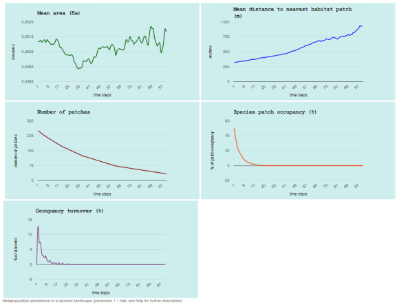
To simulate the dynamics across multiple steps and get the results use the ‘iterate.graph’ function, which runs the full simulation:
it1 <- iterate.graph(iter = 2,
                     mapsize = 10000,
                     dist_m = 10,
                     areaM = 0.05,
                     areaSD = 0.02,
                     Npatch = 250,
                     disp = 800,
                     span = 100,
                     par1 = "hab",
                     par2 = 2,
                     par3 = NULL,
                     par4 = NULL,
                     par5 = NULL,
                     method = "percentage",
                     parm = 50,
                     nsew = "none",
                     succ = "none",
                     param_df = param1,
                     kern = "op1",
                     conn = "op1",
                     colnz = "op1",
                     ext = "op1",
                     beta1 = NULL,
                     b = 1,
                     c1 = NULL,
                     c2 = NULL,
                     z = NULL,
                     R = NULL,
                     graph = TRUE)
## Completed iteration 1  of  2
## Completed iteration 2  of  2
Which will open the web browser with the following graphs:
And that’s all for now!
Thanks!
R-bloggers.com offers daily e-mail updates about R news and tutorials about learning R and many other topics. Click here if you're looking to post or find an R/data-science job.
Want to share your content on R-bloggers? click here if you have a blog, or here if you don't.