
Estimating Control Chart Constants with R
Want to share your content on R-bloggers? click here if you have a blog, or here if you don't.
In this post, I will show you how a very basic R code can be used to estimate quality control constants needed to construct X-Individuals, X-Bar, and R-Bar charts. The value of this approach is that it gives you a mechanical sense of where these constants come from and some reinforcement on their application.
If you work in a production or quality control environment, chances are you've made or seen a control chart. If you're new to control charting or need a refresher check out Understanding Statistical Process Control, Wheeler et. al. If you want to dive in and start making control charts with R, check out R packages
If your familiar with control charts, you've likely encountered cryptic alpha-numeric constants like d2, A2, E2, d3, D3, and asked,
“What are they and where do they come from?”
Short (not so satisfying) answer: They are constants you plug into formulas to determine your control limits. Their value depends on how many samplings you do at a time and the type of chart you are making. For example, if you measure the size of 5 widgets per lot of 50, then your subgroup size, n, is 5 and you should be using a set of control chart constants for n = 5.
So where do they come from and how are they calculated?
Read on.
X-Bar and X-Individuals Constants
Often, control charts represent variability in terms of the mean range, R, observed over several subgroup rather than the mean standard deviation. The table below should make the idea of subgroup range and mean range more clear.

Why range? My guess is that, historically, employees at all levels would have understood the concept of range. Range requires no special computation, just (max-min). Speculation aside, we begin our quest to understand where control constants come from with the relationship shown in Eq. 1 that the mean subgroup range is proportional to standard deviation of the individual values.

The proportionality constant between R(XSub_Grp_Indv) and S(Xindv) is d2, the first constant we'll be estimating. The relationship is expressed in Eq.2

To estimate d2 for n = 2 (i.e, the subgroup size is 2), we start by drawing two samples from a normal distribution with mean = 0 and sd = 1. Why you ask? Because it makes the math really simple. Consider Eq. 2, if S(Xindv) = 1 then R(XSub_Grp_Indv) = d2.
So all we need to do to determine d2 when n = 2 is:
- Draw 2 individuals from the normal distribution,
- Determine the range of the 2 samples.
- Repeat many, many times
- Take the average of all the ranges you’ve calculated, R
- R = d2 (when the mean = 0 and sd = 1)
The R code for the process is shown below.
```r
require(magrittr)  #Bring in the Pipe Function
reps <- 1E6
set.seed(5555)
replicate(reps, rnorm(n=2, mean = 0, sd = 1) %>% #Draw Two From the Normal Distibution
    range() %>% #Determine the Range Vector = (Max, Min)
    diff() %>% #Determine the Difference of the Range Vector
    abs() #Take the Absolution Value to make sure the Result is positive
    ) %>% # Replicate the above proceedure 1,000,000 Times
    mean() -> R_BAR -> d2 #Take the mean of the 1,000,000 ranges
d2
```

```
## [1] 1.12804
```
The pipes make the above code easy to read but slow things down quite a bit. The following code does the same thing about 12.5 times faster.
```r
reps <- 1E6
set.seed(5555)
d2 <- R_BAR <- mean(replicate(reps, abs(diff(range(rnorm(2))))))
d2
```

```
## [1] 1.12804
```
Once you have d2, calculating E2 (3σ for the individuals) and A2 (3σ for the sub-group means) is straight forward as shown in Eq.3 - Eq.6. A2 and E3 are the coefficients to the left of R.

The code below gives the expected results for all the control constants need to construct X-Bar and X-Individual charts.
```r
c(N=2, d2 = d2, E2 = 3/d2, A2 = 3/(d2*sqrt(2)))
```

```
##        N       d2       E2       A2
## 2.000000 1.128040 2.659480 1.880536
```
R-Bar Constants
The constants for R charts are d3 (1σ around R,), D3 (Lower 3σ limit of R) and D4 (Upper 3σ limit of R). To get these constants, we start with the assumption that the standard deviation of R is proportional to the standard deviation of the individual X's. The proportionality constant is d3 shown in Eq.7. Notice that Eq. 7 has the same form as Eq. 2.

```r
reps <- 1E6
set.seed(seed)
d3 <- sd(replicate(reps, abs(diff(range(rnorm(2))))))
d3
```

```
## [1] 0.8529419
```
Notice in the R code above, the only difference between the calculation of d3 and d2 is that we use standard deviation rather than the mean of the RSub_Grp_Indv. Now we have d3, but we need to do a little simple algebra to express the S(RSub_Grp_Indv) in terms of R. Remember, historically the employee doesn't need to worry about standard deviation – just ranges. We can define the above expression in term of R by combining Eq.2 and Eq.7, yielding Eq.8.

OK almost to D3 and D4. The lower 3σ limit of R can be expressed as Eq.8:

Factoring out the R terms on the right-hand side of the expression yields
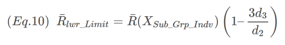
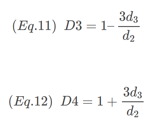
The expression inside the parentheses is D3. D4, the upper limit of R is evaluated analogously. The only difference is a “+” sign in the final expression. Final expressions for D3 and D4 are:
All done! Here is the R code summarizing the constants for R using n=2.
```r
c(N  = 2,
  d3 = d3,
  D3 = ifelse(1 - 3*d3/d2 < 0, 0, 1 - 3*d3/d2),
  D4 = 1 + 3*d3/d2
  )
```

```
##         N        d3        D3        D4
## 2.0000000 0.8529419 0.0000000 3.2683817
```
Notice for D3 the value is 0, this is because the value calculated was negative. Such values are rounded to zero per the R code above.
Summary
In this post, we used R to estimate the control chart constants needed to produce X-Individuals, X-Bar, and R-Bar charts. All the constants together are shown below. In addition, the constants for n = 7 have also been presented.
```r
reps <- 1E6
set.seed(5555)
FUN_d2 <- function(x) {mean(replicate(reps, abs(diff(range(rnorm(x))))))}
FUN_d3 <- function(x) {sd(replicate(reps, abs(diff(range(rnorm(x))))))}

Ns <- c(2,7)
d2 <- sapply(Ns, FUN_d2)
d3 <- sapply(Ns, FUN_d3)

round(data.frame(
  N = Ns,
  d2 = d2,
  E2 = 3/d2,
  A2 = 3/(d2*sqrt(Ns)),
  d3 = d3,
  D3 = ifelse(1 - 3*d3/d2 < 0, 0, 1 - 3*d3/d2),
  D4 = 1 + 3*d3/d2
  ), digits = 3)
```

```
##   N    d2    E2    A2    d3    D3    D4
## 1 2 1.128 2.659 1.881 0.854 0.000 3.272
## 2 7 2.704 1.109 0.419 0.833 0.076 1.924
```
R-bloggers.com offers daily e-mail updates about R news and tutorials about learning R and many other topics. Click here if you're looking to post or find an R/data-science job.
Want to share your content on R-bloggers? click here if you have a blog, or here if you don't.