There is interest in bitcoin at the moment because it is displaying signs of steady year to year growth with brief boosts followed by rapid declines. It is considered a risky investment by investors yet, has the potential for high returns in a fairly short duration (1-2 years). John McAfee, inventor of McAfee anti virus software has reasoned that bitcoin will reach $1,000,000 per bitcoin by 2020 (https://www.reddit.com/r/Bitcoin/comments/7w5gpa/i_made_a_website_to_track_the_mcafee_prediction_1/). Its current value is around $6000-8000. I am a data analyst working with genomic data at QMUL, I am also interested in forecasting the value of bitcoin and investing. Cryptocurrency is a step forward from fiat currencies which are without intrinsic value and subject to steady inflation. I have been using Rob Hyndman’s (https://robjhyndman.com/) R forecast package to make predictions from the time course data we have so far, this is an alternative to fitting an (probably a bit crazy) exponential model as I believe John McAfee did. This model I am using just assumes future bitcoin price is a function of past bitcoin price, and we are ignoring any outside variables. This is a big assumption, but bitcoin price does seem to have a strong underlying trend over the years.

The results and code are follows, this is a quick analysis and more work is required to build on this, I’m going to skip including the maths below as I haven’t got the time to be honest. Also required are tests to show normality of the residuals and that they are uncorrelated (this could be done with checkresiduals(fit));

First, we load the packages required and take log2 of the bitcoin price. I’ve log2 transformed the data because the bitcoin dollar prices are very unevenly distributed with lots of low values that rapidly increase (see also, https://www.reddit.com/r/Bitcoin/comments/8zxn7l/predicting_the_price_of_bitcoin/). Note, we need to use a ggplot2 custom function to produce nice looking plots from the forecast object (e.g. https://gist.github.com/fernandotenorio/3889834). I got the price data from here (https://www.coindesk.com/price/).

library(ggplot2)
library(tseries)
library(forecast)

setwd("C:/Users/chris/Desktop/investments/")
data <- read.csv('bitcoinrawdata.csv')
data$date <- as.character(data$date)
year <- sapply(strsplit(data$date, " "), `[`, 1)
data$date <- year
data$price <- log2(data$price)
data$date = as.Date(data$date, "%d/%m/%Y")
ggplot(data, aes(date,price)) + geom_point() + scale_x_date('month')

So we can see something of a hyperbolic trend of bitcoin price (in log2 dollars) with time, with these peaks which look rather non-seasonal and unpredictable. We could try and take these into account in some way, but this would add complexity, so I am just proceeding with modelling based on overall trends so far.

Now we are ready to run the prediction code. First, lets just take a look at the wikipedia entry for ARIMA (https://en.wikipedia.org/wiki/Autoregressive_integrated_moving_average).

“The AR part of ARIMA indicates that the evolving variable of interest is regressed on its own lagged (i.e., prior) values. The MA part indicates that the regression error is actually a linear combination of error terms whose values occurred contemporaneously and at various times in the past. The I (for “integrated”) indicates that the data values have been replaced with the difference between their values and the previous values (and this differencing process may have been performed more than once). The purpose of each of these features is to make the model fit the data as well as possible.”

Auto ARIMA is a nice function for lazy people such as me, because it automatically selects a model according to AIC within the universe of ARIMA models (Hyndman et al., 2007). Oftentimes automated model selection will beat a manual decision. Although, we have to consider this a very approximate prediction. Let us now run the auto.arima method from the forecast package and predict the course of bitcoin roughly over the next 4-5 years.

count_ma = ts(data$price, frequency=365, start=c(2010,07))
arima = auto.arima(count_ma)
arima <- forecast(arima, h=2427)
accuracy(arima) # RMSE 0.0836
plot(arima) + abline(h=20)
source('C:/Users/chris/Desktop/investments/plotfromforecast.R')
pg(arima)
as.numeric(arima$mean)

So we can see using just this data, if bitcoin behaves according to just the previous data and trends it will take until approximately 2022 to reach $1,000,000 per bitcoin (1 million this equals roughly 2^20 dollars which is why we look at 20 on the y axis as we are doing inverse log2). By 2020, according to this model, we will most likely be at around $65,000.

Let’s have a go with automated exponential smoothing. This is a quote from wikipedia for exponential smoothing (https://en.wikipedia.org/wiki/Exponential_smoothing).

“Exponential smoothing is a rule of thumb technique for smoothing time series data using the exponential window function. Whereas in the simple moving average the past observations are weighted equally, exponential functions are used to assign exponentially decreasing weights over time. It is an easily learned and easily applied procedure for making some determination based on prior assumptions by the user, such as seasonality.”

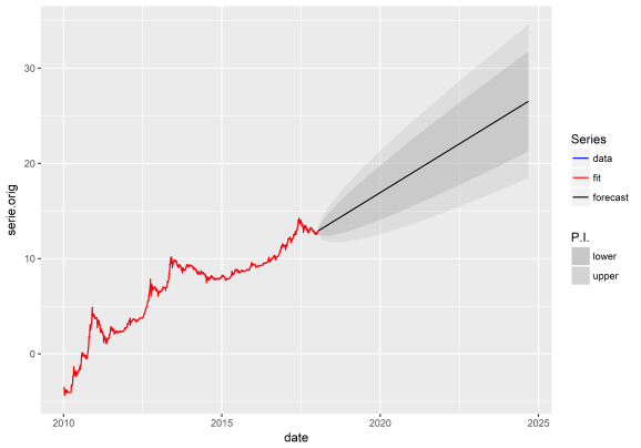
The RMSE is slightly higher here so the model does not fit the data quite as well as automated ARIMA. The prediction is slightly less optimistic as we can see we have to wait until half way through 2022 to reach $1,000,000 per bitcoin (20 on y axis). However, looking qualitatively at this plot it seems to fit with the hyperbolic trend better we are observing. More data should be insightful over the next few years.

mod_exponential <- ets(count_ma)
forecast <- forecast(mod_exponential, h = 2427)
accuracy(forecast) # RMSE 0.0839
plot(forecast)+ abline(h=20)
source('C:/Users/chris/Desktop/investments/plotfromforecast.R')
pg(forecast)

So, we can see using the CRAN forecast package, bitcoin is probably on the way up, but there are volatile fluctuations which are harder to predict. The bitcoin may be subject to market manipulation or outside competition. Other work to do would be investigating seasonality – no obvious periodicity could be discerned, however, we might want to quantify that. We also are not taking into account known variables such as the number of users, this could be approximated by user transactions or google searches, and incorperated into a model. We might want to play around with fitting a non linear model using nlm. However, a straightforward automated ARIMA approach as done here can lead to very good forecasts.

The models in this analysis really do not suggest bitcoin will be at $1,000,000 by 2020, but around $65,000 give or take. Investors will need to wait at least 2 more years, and likely more, i.e. 2022-2024 for a $1,000,000 value. Assuming that the same trends occur, i.e. user number growth. Also, this blog entry is just a bit of fun, so don’t take it too seriously.

Bitcoin is a highly risky investment, do not invest more than you would be prepared to accept losing.

This blog should hopefully also be found at: https://www.r-bloggers.com, in the near future.

References

Hyndman, Rob J., and Yeasmin Khandakar. Automatic time series for forecasting: the forecast package for R. No. 6/07. Monash University, Department of Econometrics and Business Statistics, 2007.