
Digitalization, India, New Products & Forecasting
Want to share your content on R-bloggers? click here if you have a blog, or here if you don't.
Digitalization and Demonetization
India being the land of culture, land of opportunites and land of 130 cr consumers.
Over the years, India is not able to grow to its actual potential; major roadbloack was and is corruption.
This present Indian government’s very unpopular move of Demonetization aimed to curb corruption and push India towards Digitalization.
Although demonetization created lot of havoc and problems but it also created opportunities for the new product/s.
I don’t know whether it curbed the corruption or not but I can see a clear push towards digital banking echo system and new products.

We can clearly observe during & after demonetization exponential jump of the usage of plastic money at the point of sale (POS). In December’2016, debt cards usage at POS is almost 4 times that of October usage.
We all expected that this increase will ease it out once situation become normal & new currency is easily available, even traders in India don’t encourage to take payments through plastic money as these transactions comes under income tax.
Though the situation had become normal now, usage of the plastic money at POS is still almost twice as that of before demonetization.
Mobile Money
Demonetization also created an environment where mobile cash can grow many folds and here mobile wallets and newly launched Unified payment Interface got the perfect opportunity to grow.
In October 2016, before demonetization, Mobile wallet + UPI together accounts for nearly 100 mn transactions which has now grown to 469 mn transactions in April 2018 and as per latest figures from RBI, alone UPI transactions in the month of June’18 accounts is little more than 400 mn transactions.

Trend is clearly visible – India is slowly moving towards cashless economy.
But the bigger question of an hour is do we have such infrastructure ready for such kind of transition?
Forecast for the POS machines
Here is the small attempt to predict/forecast the number POS machines required for the next 1 year.
Data source is again RBI.
Before modeling the dataset, need to follow below guidelines (Courtsey Learnings from Time series Analysis @ Coursera)
Guidelines for modeling the time series
- Trend suggests differencing
- Variation in variance suggests transformation
- Common transformation: log, then differencing -It is also known as log-return
- ACF suggests order of moving average process (q)
- PACF suggests order of autoregressive process (p)
- Akaike Information Criterion (AIC)
- Sum of squared errors (SSE)
- Ljung-Box Q-statistics
- Estimation!
library(tidyverse)
library(forecast)
library(astsa)
library(knitr)

load(file="pos_forecasting.rda")
data$Date <- as.Date(data$Date, format= "%d-%m-%Y")

#top 5 rows of the data

kable (head(data,5))
| Bank_Name | Bank_Type | Date | Number_of_POS |
|---|---|---|---|
| Allahabad Bank | Nationalised banks | 2011-04-01 | 0 |
| Andhra Bank | Nationalised banks | 2011-04-01 | 2113 |
| Bank of Baroda | Nationalised banks | 2011-04-01 | 4537 |
| Bank of India | Nationalised banks | 2011-04-01 | 2581 |
| Bank of Maharashtra | Nationalised banks | 2011-04-01 | 481 |
pos_data<-aggregate(data$Number_of_POS, by=list(data$Date), sum)

names (pos_data)<- c("Date","POS")

#converting the data in ts format

ts_pos<- ts(pos_data[,-1],start = c(2011,4),end = c(2018,5), frequency = 12)
Ploting the data to figure out the trend
plot (ts_pos, main="Monthly POS machines deployed", ylab="Number of POS Machines deployed")
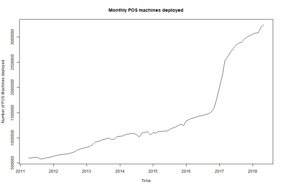
Clearly we can see their is trend in the data & series is not Stationay.
We need to remove the trend.
Lets first check is there any auto- correlation between different lags of the time series.
For this we will use Box Test.
Box.test (ts_pos,lag=log(length(ts_pos)))

Box-Pierce test
data: ts_pos
X-squared = 273.29, df = 4.4543, p-value < 2.2e-16
The p- value is very small – which indicates there is definately auto-correaltion.
Now the next step is to remove the trend, I will use difference operator (diff)
plot (diff(ts_pos),main="Diferenced data of 1st order", ylab="Number of POS Machines deployed")

Box.test (diff(ts_pos),lag=log(length(diff(ts_pos))))

Box-Pierce test
data: diff(ts_pos)
X-squared = 81.76, df = 4.4427, p-value < 2.2e-16
Still we can see the trend in the data. Again we have to apply difference operator
plot (diff(diff(ts_pos)),main="Diferenced data of order 2", ylab="Number of POS Machines deployed")

Box.test (diff(diff(ts_pos)),lag=log(length(diff(diff(ts_pos)))))

Box-Pierce test
data: diff(diff(ts_pos))
X-squared = 15.703, df = 4.4308, p-value = 0.004967
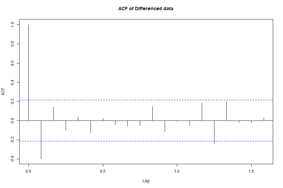
Now let’s look at the ACF & PACF which also suggest auto-correaltion in the data
acf (diff(diff(ts_pos)), main="ACF of Differenced data")
pacf(diff(diff(ts_pos)), main='PACF of differenced data')

-
ACF – There is significant lag at lag 1 and 1 pick at lag 14 (may be we can ignore this and refer this as randomness).
-
PACF – There is significant lag at lag 1 (for autoregressive process)
Now let try different models
It is clear, our d=2 (we have performed difference twice)
Now let’s figure out other parameter of ARIMA model
diff.model<- c()
mod1<- c()
d=2;z=1
for(p in 1:4){
  for(q in 1:4){
          if(p+d+q<=10){
          model<-arima(x=ts_pos, order = c((p-1),d,(q-1)))
          pval<-Box.test(model$residuals, lag=log(length(model$residuals)))
          sse<-sum(model$residuals^2)
          mod1<- c(model$aic,sse,pval$p.value)
         diff.model<- cbind(diff.model,mod1)

        }
      }
    }
colnames(diff.model)<- c ("Arima 0,2,0","Arima 0,2,1","Arima 0,2,2","Arima 0,2,3","Arima 1,2,0","Arima 1,2,1","Arima 1,2,2","Arima 1,2,3","Arima 2,2,0","Arima 2,2,1","Arima 2,2,2","Arima 2,2,3","Arima 3,2,0","Arima 3,2,1","Arima 3,2,2","Arima 3,2,3")
rownames (diff.model)=c('AIC', 'SSE', 'p-value')

kable (diff.model)
| Arima 0,2,0 | Arima 0,2,1 | Arima 0,2,2 | Arima 0,2,3 | Arima 1,2,0 | Arima 1,2,1 | Arima 1,2,2 | Arima 1,2,3 | Arima 2,2,0 | Arima 2,2,1 | Arima 2,2,2 | Arima 2,2,3 | Arima 3,2,0 | Arima 3,2,1 | Arima 3,2,2 | Arima 3,2,3 | |
|---|---|---|---|---|---|---|---|---|---|---|---|---|---|---|---|---|
| AIC | 2.04390e+03 | 2.032641e+03 | 2.034152e+03 | 2.034000e+03 | 2.031575e+03 | 2.033573e+03 | 2.034886e+03 | 2.030729e+03 | 2.033574e+03 | 2.029861e+03 | 2.031232e+03 | 2.032559e+03 | 2.035330e+03 | 2.037349e+03 | 2.032914e+03 | 2.034753e+03 |
| SSE | 1.77329e+11 | 1.511417e+11 | 1.502817e+11 | 1.460151e+11 | 1.492217e+11 | 1.492186e+11 | 1.478676e+11 | 1.360945e+11 | 1.492195e+11 | 1.379507e+11 | 1.369194e+11 | 1.357870e+11 | 1.487718e+11 | 1.488064e+11 | 1.363015e+11 | 1.360618e+11 |
| p-value | 4.31830e-03 | 8.042071e-01 | 9.096711e-01 | 9.588175e-01 | 9.737261e-01 | 9.731882e-01 | 9.171468e-01 | 9.993006e-01 | 9.733108e-01 | 9.898481e-01 | 9.964327e-01 | 9.749469e-01 | 9.756955e-01 | 9.678883e-01 | 9.879784e-01 | 9.919547e-01 |
From the above we can conclude that
- Model with least AIC is Arima 2,2,1.
- Second best model is ARIMA 1,2,3
- Third best model is ARIMA 1,2,0
Now the choice is between these 3 models.
Although there is a function in forecast library which automatically generate the parameter for least error.
library(forecast)
auto.arima(ts_pos)
Series: ts_pos
ARIMA(2,2,1)
Coefficients:
ar1 ar2 ma1
0.4638 0.2614 -0.9687
s.e. 0.1141 0.1113 0.0465
sigma2 estimated as 1.703e+09: log likelihood=-1010.93
AIC=2029.86 AICc=2030.37 BIC=2039.58
According to the above function also best model is ARIMA 2,2,1.
Now we will be using these parameters in our final model
library(astsa)

sarima(ts_pos,2,2,1,0,0,0)
initial value 10.747222
iter 2 value 10.726566
iter 3 value 10.663160
iter 4 value 10.660967
iter 5 value 10.660754
iter 6 value 10.660753
iter 7 value 10.660729
iter 8 value 10.660648
iter 9 value 10.660585
iter 10 value 10.660574
iter 11 value 10.660567
iter 12 value 10.660528
iter 13 value 10.660371
iter 14 value 10.660275
iter 15 value 10.660237
iter 16 value 10.660214
iter 17 value 10.659064
iter 18 value 10.658786
iter 19 value 10.658386
iter 20 value 10.657945
iter 21 value 10.652212
iter 22 value 10.649269
iter 23 value 10.638113
iter 24 value 10.633268
iter 25 value 10.627282
iter 26 value 10.625633
iter 27 value 10.623322
iter 28 value 10.621746
iter 29 value 10.621737
iter 30 value 10.621721
iter 30 value 10.621721
final value 10.621721
converged
initial value 10.616198
iter 2 value 10.616101
iter 3 value 10.615955
iter 4 value 10.615953
iter 5 value 10.615951
iter 6 value 10.615951
iter 6 value 10.615950
iter 6 value 10.615950
final value 10.615950
converged
 $fit
$fit
Call:
stats::arima(x = xdata, order = c(p, d, q), seasonal = list(order = c(P, D,
Q), period = S), include.mean = !no.constant, optim.control = list(trace = trc,
REPORT = 1, reltol = tol))
Coefficients:
ar1 ar2 ma1
0.4638 0.2614 -0.9687
s.e. 0.1141 0.1113 0.0465
sigma2 estimated as 1.642e+09: log likelihood = -1010.93, aic = 2029.86
$degrees_of_freedom
[1] 81
$ttable
Estimate SE t.value p.value
ar1 0.4638 0.1141 4.0652 0.0001
ar2 0.2614 0.1113 2.3494 0.0212
ma1 -0.9687 0.0465 -20.8369 0.0000
$AIC
[1] 22.28911
$AICc
[1] 22.31811
$BIC
[1] 21.37472
Looking at the residual plots, we can conculde
- There is no significant auto-correlation (ACF of Residual).
- There is no small p value – which tell us there is no signifcant auto -correlation
We can assume at this point residuals are the white noise.
So the final model will be
model<-arima(x=ts_pos,order = c(1,2,1))

plot(forecast(model))

Forecast for the next 12 months
pos_predict<- forecast(model,12)
kable (pos_predict)
| Point Forecast | Lo 80 | Hi 80 | Lo 95 | Hi 95 | |
|---|---|---|---|---|---|
| Jun 2018 | 3322859 | 3268845 | 3376873 | 3240252 | 3405467 |
| Jul 2018 | 3390114 | 3288152 | 3492077 | 3234177 | 3546052 |
| Aug 2018 | 3460657 | 3297580 | 3623734 | 3211252 | 3710061 |
| Sep 2018 | 3529929 | 3298050 | 3761808 | 3175300 | 3884558 |
| Oct 2018 | 3599692 | 3291072 | 3908312 | 3127698 | 4071685 |
| Nov 2018 | 3669265 | 3277079 | 4061451 | 3069469 | 4269061 |
| Dec 2018 | 3738912 | 3256727 | 4221096 | 3001474 | 4476349 |
| Jan 2019 | 3808530 | 3230390 | 4386669 | 2924342 | 4692718 |
| Feb 2019 | 3878159 | 3198441 | 4557877 | 2838621 | 4917697 |
| Mar 2019 | 3947784 | 3161166 | 4734401 | 2744756 | 5150812 |
| Apr 2019 | 4017410 | 3118822 | 4915999 | 2643137 | 5391684 |
| May 2019 | 4087036 | 3071626 | 5102447 | 2534100 | 5639973 |
4 mn POS machine will be required to deploy in May 2019.
In May 2016 – big 4 banks (SBI, HDFC, ICICI & Axis Bank) accounts for 75% of POS machine deployed. The same 4 banks accounts for 67% in May 2017 and 57% in May 2018. New players like RBL, corporation Banks getting very aggresive in deploying POS machines.
R-bloggers.com offers daily e-mail updates about R news and tutorials about learning R and many other topics. Click here if you're looking to post or find an R/data-science job.
Want to share your content on R-bloggers? click here if you have a blog, or here if you don't.