Getting and parsing data with AWK

Currency exchange rate data (ARS / USD)

Hi everyone! This is our first post in this new blog!
We imagine that it is going to be the first one in a series about time series, a time series itself!
So we are going to start from the very beginning!

First, obviously we need a question to ask, a problem to solve or something as vague as it could be to make possible to us to follow this beautiful natural disorder. Once we pick up this Ariadne’s thread we start to pull it towards us or following towards its origin, both the length of the thread and where it goes are unknown to us.

So we pick up a very notorious thread in our Argentinean society. The price of the US dollar and its parity with our local currency the “Peso Argentino” is known as the exchange rate. This subject is a very polemical one so we are going to get actual data to better understand what’s happening with it.

Well, our problem is a very common one. We don’t know really what money is. We know that we have some money in our pockets, that this money is usually in the form of notes and these pieces of paper could be used to turn you in a crazy consumerist, to sink you down in the lowest and cruelest parts of society or to buy some bananas. It’s certainly madness. But if we accept (or not) that we can’t escape from this crazy reality we need to begin at least to understand it.

So, it seems that currencies have some kind of ‘strength’ and obviously since strength is a word that refers to something relative, then we could assume that we can measure it. One of these measures that’s usually used in our economy is the price of the US dollar, put simply, how many US dollars you can buy with an Argentine Peso.

Ok, let’s finish with the introduction and let’s grab some real data. First we started using Google to explore where could we get some data. Our first guess was to go directly to the sources, either to our Central Bank or to our National Bank. In their website we could see that we could get the data we were looking for but unfortunately we just were able to get it by one day at time. For example you could ask the exchange rate for any day from here to 1993 but only one day. So in order to get a series of, maybe 365 times 20 years we needed to repeat this process 7300 times. This is a very impractical thing to do, Therefore our friends in our National Bank weren’t helpful to us. But luckily we found that someone is collecting this data here and in there we had the possibility of getting a HTML table of historical values.

Then we got an .HTML table with our data since year 2000, we downloaded this page and then we used AWK to parse it and printed it to a .csv file for its use in R!. The following flowchart briefly summarizes this post.

The AWK script and its explanation as well are available in our Github.

Using R

Once we had our data, we read it and converted the raw dates to date objects in R and made some initial visualizations of the data. Also the whole script can be found here.

# Read data
dataDolar <- read.csv("../data/data_peso_dolar.csv")
# Converting to an object of class date
dataDolar$fecha <- as.Date(dataDolar$fecha, "%d/%m/%Y")
plot(x = dataDolar$fecha,
     y = dataDolar$divisa_venta,
     type = "l",
     xlab="Date",
     ylab="Argentine Peso / US Dollar")

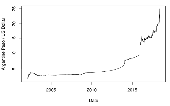
We can see in this first plot that the tendency is obviously rising and it has some recent spikes. But we need to get some more complementary data to better understand it. For example, one first approximation to it could be to know which president has been in office for each period observed.

To do that we got this information from the great Wikipedia!

Because we are from Argentina and we are a bit scared and traumatized by some dark periods in our recent history we ignored the period before the Nestor Kirchner’s presidency. For now. Later on we’ll get deeper on these obscure times!

Ok, let’s then to get our hands dirty again on R!

And now we have a new variable as factor that corresponds to which president was or is now in office.

So, finishing our first exploratory data visualizations we are going to make the same plot as before but with some supplementary data in it.

# Choose the colors
colores <- c("orange3",  "steelblue4", "red","yellowgreen","gray20")
# Set the colors
palette(colores)
# Plot
plot(x = dataDolar$fecha,
     y = dataDolar$divisa_venta,
     xlab="Date",
     ylab="Argentine Peso / US Dollar",
     type="p",
     col=dataDolar$Presidencia,
     cex=0.25)
# Add legend
legend("topleft", legend = levels(dataDolar$Presidencia),
       col = 1:5,
       lwd = c(3,3,3,3),
       cex = 0.75,
       box.lty = 0)

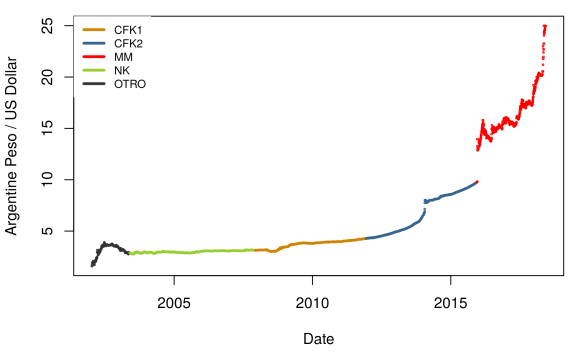
So now we have some ideas of what happened and what’s happening right now with our Peso! But we need to go deeper, in the next editions of this series we’ll see much more!
See you all until the next post!