
Data transformation in #tidyverse style: package sjmisc updated #rstats
Want to share your content on R-bloggers? click here if you have a blog, or here if you don't.
I’m pleased to announce an update for the sjmisc-package, which was just released on CRAN. Here I want to point out two important changes in the package.
New default option for recoding and transformation functions
First, a small change in the code with major impact on the workflow, as it affects argument defaults and is likely to break your existing code – if you’re using sjmisc: The append-argument in recode and transformation functions like rec(), dicho(), split_var(), group_var(), center(), std(), recode_to(), row_sums(), row_count(), col_count() and row_means() now defaults to TRUE.
The reason behind this change is that, in my experience and workflow, when transforming or recoding variables, I typically want to add these new variables to an existing data frame by default. Especially in a pipe-workflow, when I start my scripts with importing and basic tidying of my data, I almost always want to append the recoded variables to my existing data, e.g.:
# Example with following steps:
# 1. loading labelled data set
# 2. dropping unused labels
# 3. converting numeric into categorical, using labels as levels
# 4. center some variables
# 5. recode some other variables
data %>%
  drop_labels() %>%
  as_label(var1:var5) %>%
  center(var7, var9) %>%
  rec(var11, rec = "2=0;1=1;else=copy")
The above code would return a data frame with 3 new, additional variables, var7_c and var9_c (centered) and var11_r (recoded).
In the past package versions, the append-argument defaulted to FALSE, which means that functions like rec() or center() did not return the input data frame including the new variables, but only the new, transformed variables. This was a behaviour that turned out to be less practical as default option.
Freak out
The second change is a revision of the frq() function, which prints frequency tables in a clean and well-arranged way to console (or as HTML table). frq() now prints more summary statistics in the headline, as well as the variable name and type:
library(tidyverse)
library(strengejacke)
# Get pkg "strengejacke" from Github:
# https://github.com/strengejacke/strengejacke
# it simply loads 4 of my packages at once...

data(efc)
frq(efc, e42dep, e15relat)

#> # elder's dependency (e42dep) <numeric>
#> # total N=908  valid N=901  mean=2.94  sd=0.94
#>
#>  val                label frq raw.prc valid.prc cum.prc
#>    1          independent  66    7.27      7.33    7.33
#>    2   slightly dependent 225   24.78     24.97   32.30
#>    3 moderately dependent 306   33.70     33.96   66.26
#>    4   severely dependent 304   33.48     33.74  100.00
#>   NA                   NA   7    0.77        NA      NA
#>
#>
#> # relationship to elder (e15relat) <numeric>
#> # total N=908  valid N=901  mean=2.85  sd=2.08
#>
#>  val                   label frq raw.prc valid.prc cum.prc
#>    1          spouse/partner 171   18.83     18.98   18.98
#>    2                   child 473   52.09     52.50   71.48
#>    3                 sibling  29    3.19      3.22   74.69
#>    4 daughter or son -in-law  85    9.36      9.43   84.13
#>    5              ancle/aunt  23    2.53      2.55   86.68
#>    6            nephew/niece  22    2.42      2.44   89.12
#>    7                  cousin   6    0.66      0.67   89.79
#>    8          other, specify  92   10.13     10.21  100.00
#>   NA                      NA   7    0.77        NA      NA
For non-labelled data, like the iris dataset, frq() no longer prints an empty label column, and the variable name is also printed in the headline:
data(iris)
frq(iris, Species)

#> # Species <categorical>
#> # total N=150  valid N=150  mean=2.00  sd=0.82
#>
#>         val frq raw.prc valid.prc cum.prc
#>      setosa  50   33.33     33.33   33.33
#>  versicolor  50   33.33     33.33   66.67
#>   virginica  50   33.33     33.33  100.00
#>           0    0.00        NA      NA
Furthermore, it’s now possible to automatically group variables with a large range of value. In this example, you see the difference between the frequency tables of a variable containing information on age. The auto.grp-argument takes a numeric value, which indicates at which amount of different unique values a variable is grouped. For instance, if auto.grp = 5, variables with more than 5 unique values are recoded into 5 groups (of same range).
frq(efc, e17age)

#> # elder' age (e17age) <numeric>
#> # total N=908  valid N=891  mean=79.12  sd=8.09
#>
#>   val frq raw.prc valid.prc cum.prc
#>    65  32    3.52      3.59    3.59
#>    66  24    2.64      2.69    6.29
#>    67  29    3.19      3.25    9.54
#>    68  24    2.64      2.69   12.23
#>    69  29    3.19      3.25   15.49
#>    70  32    3.52      3.59   19.08
#>    71  20    2.20      2.24   21.32
#>    72  22    2.42      2.47   23.79
#>    73  34    3.74      3.82   27.61
#>    74  28    3.08      3.14   30.75
#>    75  37    4.07      4.15   34.90
#>    76  37    4.07      4.15   39.06
#>    77  31    3.41      3.48   42.54
#>    78  30    3.30      3.37   45.90
#>    79  46    5.07      5.16   51.07
#>    80  34    3.74      3.82   54.88
#>    81  33    3.63      3.70   58.59
#>    82  46    5.07      5.16   63.75
#>    83  43    4.74      4.83   68.57
#>    84  43    4.74      4.83   73.40
#>    85  24    2.64      2.69   76.09
#>    86  34    3.74      3.82   79.91
#>    87  28    3.08      3.14   83.05
#>    88  19    2.09      2.13   85.19
#>    89  32    3.52      3.59   88.78
#>    90  24    2.64      2.69   91.47
#>    91  20    2.20      2.24   93.71
#>    92  13    1.43      1.46   95.17
#>    93  15    1.65      1.68   96.86
#>    94  12    1.32      1.35   98.20
#>    95   7    0.77      0.79   98.99
#>    96   1    0.11      0.11   99.10
#>    97   5    0.55      0.56   99.66
#>    98   1    0.11      0.11   99.78
#>    99   1    0.11      0.11   99.89
#>   103   1    0.11      0.11  100.00
#>    17    1.87        NA      NA

frq(efc, e17age, auto.grp = 5)

#> # elder' age (e17age) <numeric>
#> # total N=908  valid N=891  mean=79.12  sd=8.09
#>
#>  val  label frq raw.prc valid.prc cum.prc
#>    1  65-72 212   23.35     23.79   23.79
#>    2  73-80 277   30.51     31.09   54.88
#>    3  81-88 270   29.74     30.30   85.19
#>    4  89-96 124   13.66     13.92   99.10
#>    5 97-104   8    0.88      0.90  100.00
#>   NA     NA  17    1.87        NA      NA
Finally, frq() better deals with string data. Especially for open answer questions, in large datasets, a frequency table of string values can be very large. The show.strings argument allows you to omit string values from the output. Furthermore, grp.strings allows you to group “similar” strings, which is useful for open answers which slightly differ in their spelling, but actually would mean the same thing.
This first example omits the string variables:
data(mtcars)
tmp <- rownames_to_column(mtcars)

# prints only 2nd variable, because first variable
# is a string variable with rownames
frq(tmp, 1:2, show.strings = FALSE)

#> # mpg <numeric>
#> # total N=32  valid N=32  mean=20.09  sd=6.03
#>
#>   val frq raw.prc valid.prc cum.prc
#>  10.4   2    6.25      6.25    6.25
#>  13.3   1    3.12      3.12    9.38
#>  14.3   1    3.12      3.12   12.50
#>  14.7   1    3.12      3.12   15.62
#>    15   1    3.12      3.12   18.75
#>  15.2   2    6.25      6.25   25.00
#>  15.5   1    3.12      3.12   28.12
#>  15.8   1    3.12      3.12   31.25
#>
#>     0    0.00        NA      NA
The next examples includes all variables.
# prints both variables
frq(tmp, 1:2, show.strings = TRUE)

#> # rowname <character>
#> # total N=32  valid N=32  mean=16.50  sd=9.38
#>
#>                  val frq raw.prc valid.prc cum.prc
#>          AMC Javelin   1    3.12      3.12    3.12
#>   Cadillac Fleetwood   1    3.12      3.12    6.25
#>           Camaro Z28   1    3.12      3.12    9.38
#>    Chrysler Imperial   1    3.12      3.12   12.50
#>           Datsun 710   1    3.12      3.12   15.62
#>     Dodge Challenger   1    3.12      3.12   18.75
#>           Duster 360   1    3.12      3.12   21.88
#>         Ferrari Dino   1    3.12      3.12   25.00
#>             Fiat 128   1    3.12      3.12   28.12
#>            Fiat X1-9   1    3.12      3.12   31.25
#>       Ford Pantera L   1    3.12      3.12   34.38
#>          Honda Civic   1    3.12      3.12   37.50
#>       Hornet 4 Drive   1    3.12      3.12   40.62
#>    Hornet Sportabout   1    3.12      3.12   43.75
#>  Lincoln Continental   1    3.12      3.12   46.88
#>         Lotus Europa   1    3.12      3.12   50.00
#>        Maserati Bora   1    3.12      3.12   53.12
#>            Mazda RX4   1    3.12      3.12   56.25
#>        Mazda RX4 Wag   1    3.12      3.12   59.38
#>             Merc 230   1    3.12      3.12   62.50
#>            Merc 240D   1    3.12      3.12   65.62
#>             Merc 280   1    3.12      3.12   68.75
#>            Merc 280C   1    3.12      3.12   71.88
#>           Merc 450SE   1    3.12      3.12   75.00
#>           Merc 450SL   1    3.12      3.12   78.12
#>          Merc 450SLC   1    3.12      3.12   81.25
#>
#>                    0    0.00        NA      NA
#>
#>
#> # mpg <numeric>
#> # total N=32  valid N=32  mean=20.09  sd=6.03
#>
#>   val frq raw.prc valid.prc cum.prc
#>  10.4   2    6.25      6.25    6.25
#>  13.3   1    3.12      3.12    9.38
#>  14.3   1    3.12      3.12   12.50
#>  14.7   1    3.12      3.12   15.62
#>    15   1    3.12      3.12   18.75
#>  15.2   2    6.25      6.25   25.00
#>  15.5   1    3.12      3.12   28.12
#>
#>     0    0.00        NA      NA
Finally the example on how to group similar string values.
# group similar strings
frq(tmp, 1, grp.strings = 3)

#> # rowname <character>
#> # total N=32  valid N=32  mean=14.19  sd=7.13
#>
#>                                       val frq raw.prc valid.prc cum.prc
#>                               AMC Javelin   1    3.12      3.12    3.12
#>                        Cadillac Fleetwood   1    3.12      3.12    6.25
#>                                Camaro Z28   1    3.12      3.12    9.38
#>                         Chrysler Imperial   1    3.12      3.12   12.50
#>                                Datsun 710   1    3.12      3.12   15.62
#>                          Dodge Challenger   1    3.12      3.12   18.75
#>                                Duster 360   1    3.12      3.12   21.88
#>                              Ferrari Dino   1    3.12      3.12   25.00
#>                       Fiat 128, Fiat X1-9   2    6.25      6.25   31.25
#>                            Ford Pantera L   1    3.12      3.12   34.38
#>                               Honda Civic   1    3.12      3.12   37.50
#>                            Hornet 4 Drive   1    3.12      3.12   40.62
#>                         Hornet Sportabout   1    3.12      3.12   43.75
#>                       Lincoln Continental   1    3.12      3.12   46.88
#>                              Lotus Europa   1    3.12      3.12   50.00
#>                             Maserati Bora   1    3.12      3.12   53.12
#>                                 Mazda RX4   1    3.12      3.12   56.25
#>                             Mazda RX4 Wag   1    3.12      3.12   59.38
#>  Merc 230, Merc 240D, Merc 280, Merc 280C   4   12.50     12.50   71.88
#>       Merc 450SE, Merc 450SL, Merc 450SLC   3    9.38      9.38   81.25
#>                          Pontiac Firebird   1    3.12      3.12   84.38
#>                             Porsche 914-2   1    3.12      3.12   87.50
#>             Toyota Corolla, Toyota Corona   2    6.25      6.25   93.75
#>                                   Valiant   1    3.12      3.12   96.88
#>                                Volvo 142E   1    3.12      3.12  100.00
#>                                         0    0.00        NA      NA
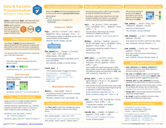
Cheat Sheet
Along with the package, I also updated the cheat sheet.
Finally
Feedback or suggestions are always welcome! Please use the dedicated GitHub page to submit an issue…
R-bloggers.com offers daily e-mail updates about R news and tutorials about learning R and many other topics. Click here if you're looking to post or find an R/data-science job.
Want to share your content on R-bloggers? click here if you have a blog, or here if you don't.