
Volatility modelling in R exercises (Part-1)
Want to share your content on R-bloggers? click here if you have a blog, or here if you don't.
Volatility modelling is typically used for high frequency financial data. Asset returns are typically uncorrelated while the variation of asset prices (volatility) tends to be correlated across time.
In this exercise set we will use the rugarch package (package description: here) to implement the ARCH (Autoregressive Conditional Heteroskedasticity) model in R.
Answers to the exercises are available here.
Exercise 1
Load the rugarch package and the dmbp dataset (Bollerslev, T. and Ghysels, E. 1996, Periodic Autoregressive Conditional Heteroscedasticity, Journal
of Business and Economic Statistics, 14, 139–151). This dataset has daily logarithmic nominal returns for Deutsche-mark / Pound. There is also a dummy variable to indicate non-trading days.
Exercise 2
Define the daily return as a time series variable and plot the return against time. Notice the unpredictability apparent from the graph.
Exercise 3
Plot the graph of the autocorrelation function of returns. Notice that there is hardly any evidence of autocorrelation of returns.
Exercise 4
Plot the graph of the autocorrelation function of squared returns. Notice the apparent strong serial correlation.
- Avoid model over-fitting using cross-validation for optimal parameter selection
- Explore maximum margin methods such as best penalty of error term support vector machines with linear and non-linear kernels.
- And much more
Exercise 5
We will first simulate and analyze an ARCH process. Use the ugarchspec function to define an ARCH(1) process. The return has a simple mean specification with mean=0. The variance follows as AR-1 process with constant=0.2 and AR-1 coefficient = 0.7.
Exercise 6
Simulate the ARCH process for 500 time periods. Exercises 7 to 9 use this simulated data.
Exercise 7
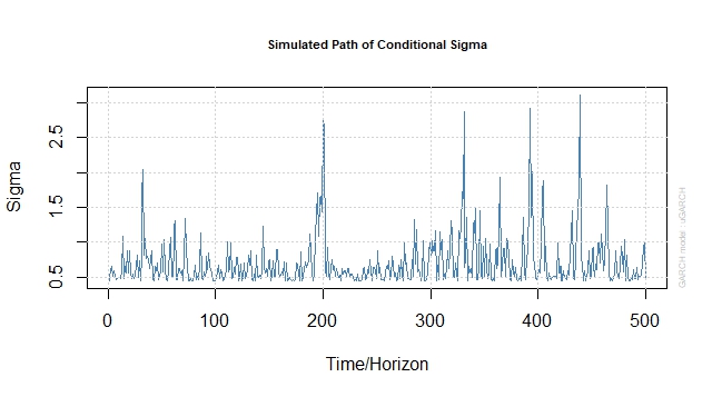
Plot the returns vs time and note the apparent unpredictability. Plot the path of conditional sigma vs time and note that there is some persistence over time.
Exercise 8
Plot the ACF of returns and squared returns. Note that there is no auto-correlation between returns but squared returns have significant first degree autocorrelation as we defined in exercise-5.
Exercise 9
Test for ARCH effects using the Ljung Box test for the simulated data.
Exercise 10
Test for ARCH effects using the Ljung Box test for the currency returns data.
R-bloggers.com offers daily e-mail updates about R news and tutorials about learning R and many other topics. Click here if you're looking to post or find an R/data-science job.
Want to share your content on R-bloggers? click here if you have a blog, or here if you don't.