
Stock Trading Analytics and Optimization in Python with PyFolio, R’s PerformanceAnalytics, and backtrader
Want to share your content on R-bloggers? click here if you have a blog, or here if you don't.
Introduction
Having figured out how to perform walk-forward analysis in Python with backtrader, I want to have a look at evaluating a strategy’s performance. So far, I have cared about only one metric: the final value of the account at the end of a backtest relative. This should not be the only metric considered. Most people care not only about how much money was made but how much risk was taken on. People are risk-averse; one of finance’s leading principles is that higher risk should be compensated by higher returns. Thus many metrics exist that adjust returns for how much risk was taken on. Perhaps when optimizing only with respect to the final return of the strategy we end up choosing highly volatile strategies that lead to huge losses in out-of-sample data. Adjusting for risk may lead to better strategies being chosen.
In this article I will be looking more at backtrader‘s Analyzers. These compute metrics for strategies after a backtest that users can then review. We can easily add an Analyzer to a Cerebro instance, backtrader already comes with many useful Analyzers computing common statistics, and creating a new Analyzer for a new statistic is easy to do. Additionally, backtrader allows for PyFolio integration, if PyFolio is more to your style.
I review these methods here.
backtrader Analyzers
Let’s start by picking up where we left off. Most of this code resembles my code from previous articles, though I made some (mostly cosmetic) improvements, such as to the strategy SMAC. I also import everything I will be needing in this article at the very beginning.
from sklearn.model_selection import TimeSeriesSplit
from sklearn.utils import indexable
from sklearn.utils.validation import _num_samples
import numpy as np
import backtrader as bt
import backtrader.indicators as btind
import backtrader.analyzers as btanal
import datetime as dt
import pandas as pd
import pandas_datareader as web
from pandas import Series, DataFrame
import random
import pyfolio as pf
from copy import deepcopy

from rpy2.robjects.packages import importr

pa = importr("PerformanceAnalytics")    # The R package PerformanceAnalytics, containing the R function VaR

from rpy2.robjects import numpy2ri, pandas2ri
numpy2ri.activate()
pandas2ri.activate()


class SMAC(bt.Strategy):
    """A simple moving average crossover strategy; crossing of a fast and slow moving average generates buy/sell
       signals"""
    params = {"fast": 20, "slow": 50,                  # The windows for both fast and slow moving averages
              "optim": False, "optim_fs": (20, 50)}    # Used for optimization; equivalent of fast and slow, but a tuple
                                                       # The first number in the tuple is the fast MA's window, the
                                                       # second the slow MA's window

    def __init__(self):
        """Initialize the strategy"""

        self.fastma = dict()
        self.slowma = dict()
        self.cross  = dict()

        if self.params.optim:    # Use a tuple during optimization
            self.params.fast, self.params.slow = self.params.optim_fs    # fast and slow replaced by tuple's contents

        if self.params.fast > self.params.slow:
            raise ValueError(
                "A SMAC strategy cannot have the fast moving average's window be " + \
                 "greater than the slow moving average window.")

        for d in self.getdatanames():

            # The moving averages
            self.fastma[d] = btind.SimpleMovingAverage(self.getdatabyname(d),      # The symbol for the moving average
                                                       period=self.params.fast,    # Fast moving average
                                                       plotname="FastMA: " + d)
            self.slowma[d] = btind.SimpleMovingAverage(self.getdatabyname(d),      # The symbol for the moving average
                                                       period=self.params.slow,    # Slow moving average
                                                       plotname="SlowMA: " + d)

            # This is different; this is 1 when fast crosses above slow, -1 when fast crosses below slow, 0 o.w.
            self.cross[d] = btind.CrossOver(self.fastma[d], self.slowma[d], plot=False)

    def next(self):
        """Define what will be done in a single step, including creating and closing trades"""
        for d in self.getdatanames():    # Looping through all symbols
            pos = self.getpositionbyname(d).size or 0
            if pos == 0:    # Are we out of the market?
                # Consider the possibility of entrance
                if self.cross[d][0] > 0:    # A buy signal
                    self.buy(data=self.getdatabyname(d))

            else:    # We have an open position
                if self.cross[d][0]  cash:
                return 0    # Not enough money for this trade
            else:
                return shares

        else:    # Selling
            return self.broker.getposition(data).size    # Clear the position


class AcctValue(bt.Observer):
    alias = ('Value',)
    lines = ('value',)

    plotinfo = {"plot": True, "subplot": True}

    def next(self):
        self.lines.value[0] = self._owner.broker.getvalue()    # Get today's account value (cash + stocks)


class AcctStats(bt.Analyzer):
    """A simple analyzer that gets the gain in the value of the account; should be self-explanatory"""

    def __init__(self):
        self.start_val = self.strategy.broker.get_value()
        self.end_val = None

    def stop(self):
        self.end_val = self.strategy.broker.get_value()

    def get_analysis(self):
        return {"start": self.start_val, "end": self.end_val,
                "growth": self.end_val - self.start_val, "return": self.end_val / self.start_val}


class TimeSeriesSplitImproved(TimeSeriesSplit):
    """Time Series cross-validator
    Provides train/test indices to split time series data samples
    that are observed at fixed time intervals, in train/test sets.
    In each split, test indices must be higher than before, and thus shuffling
    in cross validator is inappropriate.
    This cross-validation object is a variation of :class:`KFold`.
    In the kth split, it returns first k folds as train set and the
    (k+1)th fold as test set.
    Note that unlike standard cross-validation methods, successive
    training sets are supersets of those that come before them.
    Read more in the :ref:`User Guide `.
    Parameters
    ----------
    n_splits : int, default=3
        Number of splits. Must be at least 1.
    Examples
    --------
    >>> from sklearn.model_selection import TimeSeriesSplit
    >>> X = np.array([[1, 2], [3, 4], [1, 2], [3, 4]])
    >>> y = np.array([1, 2, 3, 4])
    >>> tscv = TimeSeriesSplit(n_splits=3)
    >>> print(tscv)  # doctest: +NORMALIZE_WHITESPACE
    TimeSeriesSplit(n_splits=3)
    >>> for train_index, test_index in tscv.split(X):
    ...    print("TRAIN:", train_index, "TEST:", test_index)
    ...    X_train, X_test = X[train_index], X[test_index]
    ...    y_train, y_test = y[train_index], y[test_index]
    TRAIN: [0] TEST: [1]
    TRAIN: [0 1] TEST: [2]
    TRAIN: [0 1 2] TEST: [3]
    >>> for train_index, test_index in tscv.split(X, fixed_length=True):
    ...     print("TRAIN:", train_index, "TEST:", test_index)
    ...     X_train, X_test = X[train_index], X[test_index]
    ...     y_train, y_test = y[train_index], y[test_index]
    TRAIN: [0] TEST: [1]
    TRAIN: [1] TEST: [2]
    TRAIN: [2] TEST: [3]
    >>> for train_index, test_index in tscv.split(X, fixed_length=True,
    ...     train_splits=2):
    ...     print("TRAIN:", train_index, "TEST:", test_index)
    ...     X_train, X_test = X[train_index], X[test_index]
    ...     y_train, y_test = y[train_index], y[test_index]
    TRAIN: [0 1] TEST: [2]
    TRAIN: [1 2] TEST: [3]

    Notes
    -----
    When ``fixed_length`` is ``False``, the training set has size
    ``i * train_splits * n_samples // (n_splits + 1) + n_samples %
    (n_splits + 1)`` in the ``i``th split, with a test set of size
    ``n_samples//(n_splits + 1) * test_splits``, where ``n_samples``
    is the number of samples. If fixed_length is True, replace ``i``
    in the above formulation with 1, and ignore ``n_samples %
    (n_splits + 1)`` except for the first training set. The number
    of test sets is ``n_splits + 2 - train_splits - test_splits``.
    """

    def split(self, X, y=None, groups=None, fixed_length=False,
              train_splits=1, test_splits=1):
        """Generate indices to split data into training and test set.
        Parameters
        ----------
        X : array-like, shape (n_samples, n_features)
            Training data, where n_samples is the number of samples
            and n_features is the number of features.
        y : array-like, shape (n_samples,)
            Always ignored, exists for compatibility.
        groups : array-like, with shape (n_samples,), optional
            Always ignored, exists for compatibility.
        fixed_length : bool, hether training sets should always have
            common length
        train_splits : positive int, for the minimum number of
            splits to include in training sets
        test_splits : positive int, for the number of splits to
            include in the test set
        Returns
        -------
        train : ndarray
            The training set indices for that split.
        test : ndarray
            The testing set indices for that split.
        """
        X, y, groups = indexable(X, y, groups)
        n_samples = _num_samples(X)
        n_splits = self.n_splits
        n_folds = n_splits + 1
        train_splits, test_splits = int(train_splits), int(test_splits)
        if n_folds > n_samples:
            raise ValueError(
                ("Cannot have number of folds ={0} greater"
                 " than the number of samples: {1}.").format(n_folds,
                                                             n_samples))
        if (n_folds - train_splits - test_splits)  0 and test_splits > 0):
            raise ValueError(
                ("Both train_splits and test_splits must be positive"
                 " integers."))
        indices = np.arange(n_samples)
        split_size = (n_samples // n_folds)
        test_size = split_size * test_splits
        train_size = split_size * train_splits
        test_starts = range(train_size + n_samples % n_folds,
                            n_samples - (test_size - split_size),
                            split_size)
        if fixed_length:
            for i, test_start in zip(range(len(test_starts)),
                                     test_starts):
                rem = 0
                if i == 0:
                    rem = n_samples % n_folds
                yield (indices[(test_start - train_size - rem):test_start],
                       indices[test_start:test_start + test_size])
        else:
            for test_start in test_starts:
                yield (indices[:test_start],
                    indices[test_start:test_start + test_size])
Let’s create a Cerebro instance with everything added save for the analyzers.
start = dt.datetime(2010, 1, 1)
end = dt.datetime(2016, 10, 31)
symbols = ["AAPL", "GOOG", "MSFT", "AMZN", "YHOO", "SNY", "VZ", "IBM", "HPQ", "QCOM", "NVDA"]
datafeeds = {s: web.DataReader(s, "google", start, end) for s in symbols}
for df in datafeeds.values():
    df["OpenInterest"] = 0    # PandasData reader expects an OpenInterest column;
                              # not provided by Google and we don't use it so set to 0

cerebro = bt.Cerebro(stdstats=False)

plot_symbols = ["AAPL", "GOOG", "NVDA"]
is_first = True
#plot_symbols = []
for s, df in datafeeds.items():
    data = bt.feeds.PandasData(dataname=df, name=s)
    if s in plot_symbols:
        if is_first:
            data_main_plot = data
            is_first = False
        else:
            data.plotinfo.plotmaster = data_main_plot
    else:
        data.plotinfo.plot = False
    cerebro.adddata(data)

cerebro.broker.setcash(1000000)
cerebro.broker.setcommission(0.02)
cerebro.addstrategy(SMAC)
cerebro.addobserver(AcctValue)
cerebro.addobservermulti(bt.observers.BuySell)
cerebro.addsizer(PropSizer)
We add Analyzer objects to Cerebro instances with the addanalyzer() method. The objects collect data while the strategy is running then produce final statistics that users can then review by calling the Analyzer‘s get_analysis() method. These objects are intended to be light-weight, containing only the statistics requested and not the data used to generate the statistics. Usually they return ordered dictionaries containing the statics computed for the strategy.
Some of the built-in analyzers I use include:
TradeAnalyzer: This computes trade statistics, such as the number of open and closed trades, total and average profit/loss from trades, how long trades are in the market, the longest streaks (successive winning or losing trades), and other similar statistics.Returns: This computes total, average, compound, and annualized (normalized to represent returns over a year) returns, which is the growth of the portfolio.DrawDown: This computes drawdown statistics. Drawdown is how much the value of an investment or account decreases after reaching a new high, from “peak” (the high point) to “trough” (the low point). Investors and traders dislike high drawdown, and thus are interested in metrics such as the average drawdown, the maximum draw down (the biggest gap between peak and trough), and the average and maximum length of a drawdown period (which is the period between a new high and the previous high), which this analyzer computes. Traders would like average drawdowns to be small and don’t want to wait long for the next high to be reached. (Traders often cite maximum drawdown, but beware; as the timeframe increases, maximum drawdown, by definition, can only increase, and thus should not be interpreted separately from the duration of time considered.)
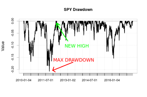
SPY max drawdown from January 2010 to June 2017, with maximum drawdown and a new peak illustrated. I created this chart using Google Finance data obtained in R via quantmod and using PerformanceAnalytics.
SharpeRatio_A: This computes the annualized Sharpe ratio. The Sharpe ratio is the most common risk-adjusted performance measure of an investment used. It is excess returns (which is return on investment minus the “risk-free” rate of return, the latter often being the return of some US government debt instruments such as T-bills) divided by the standard deviation of the returns of the investment. The higher the Sharpe ratio, the better the return of the investment relative to its volatility (which is the type of risk considered). The annualized variant of the Sharpe ratio simply annualizes the metrics used in the computation.
I attempted to use another analyzer, AnnualReturn, which computes annualized return metrics, but unfortunately it does not seem to work.
These analyzers are all useful, but we can easily create custom ones for new performance metrics not already implemented by subclassing from the Analyzer class. I did this in my blog post on walk-forward analysis. Usually creating a new analyzer involves:
- Creating modifiable parameters with a
paramsdictionary declared at the beginning of the definition of the new analyzer - Defining an
__init__()method setting up any variables needed when the analyzer is created or the backtest starts - Defining a
next()method that gets any information needed during the backtest - Defining a
stop()method for final computations - Defining a
get_analysis()method that a user can call after a backtest that returns, say, a dictionary with all the statistics the analyzer computed
In truth, only the __init__(), stop(), and get_analysis() methods are truly needed for an analyzer. Furthermore, analyzers should be light-weight; they do not need to include the entire backtest’s data to work after the backtest is completed.
Using R’s PerformanceAnalytics Package in Python
I have complaints about quantstrat, the most notable backtesting package for R, but R has many other packages useful for finance, such as quantmod or PerformanceAnalytics. In particular, PerformanceAnalytics has a lot of analytics functions not provided by backtrader and likely without a Python equivalent.
Fortunately we can easily create a backtrader Analyzer that uses PerformanceAnalytics functions. I used the following template:
- Interface with R using rpy2, an excellent R interface for Python that gives Python users access to R functions
- Use
importr()to import the R package needed (in this case, PerformanceAnalytics), and usenumpy2riandpandas2riso that NumPyndarrays and pandasSeriesandDataFrames can be translated into their R equivalents - In the
Analyzer, record the data of interest in thenext()method so that it can be transformed into a pandasSeriescontaining a time series, with adict - In the
stop()method, transform thisdictinto aSeries, then use the R function from the imported library to compute the desired metric, passing the function theSeriesof data (this will be interpreted as an R vector, which can also be interpreted as an Rtstime series thanks to the date index) - Save the results and delete the
dictof data since it is no longer needed, and inget_analysis(), just return adictcontaining the resulting calculation.
rpy2 integrates R objects quite well, using a familiar Python-like interface. pandas, being initially inspired by R, also integrates well. In fact, the pandas objects Series and DataFrame were designed initially for storing and manipulating time series data, so do as well a job as, say, R’s xts package.
Here, I use PerformanceAnalytics to create analyzers calculating two more metrics not provided by backtrader. They are:
VaR: This computes value at risk (abbreviated VaR, and the capitalization here matters, distinguishing value at risk from variance and vector autoregression, which are abbreviated with var and VAR respectively). Value at risk measures the potential loss a portfolio could see. Different ways to precisely define and calculate VaR exist, but in spirit they all give how much money could be lost at a certain likelihood. For example, if the daily 95% VaR for a portfolio is -1%, then 95% of the time the portfolio’s daily return will exceed -1% (a loss of 1%), or 5% of the time losses will exceed 1% of the portfolio’s value. This could be useful information for, say, position sizing. ThisAnalyzeris based on PerformanceAnalyticsVaRfunction.SortinoRatio: This computes the account’s Sortino ratio. The Sortino ratio is another risk-adjusted performance metric often presented as an alternative to the Sharpe ratio. It’s like the Sharpe ratio, but instead of dividing by the standard deviation of returns–which could punish volitility in the positive direction, which earns money–excess returns are divided by the standard deviation of losses alone. This is based on the PerformanceAnalytics functionSortinoRatio.
My analyzers work with log returns, or  - \log(x_{t - 1})")
class VaR(bt.Analyzer):
    """
    Computes the value at risk metric for the whole account using the strategy, based on the R package
    PerformanceAnalytics VaR function
    """
    params = {
        "p": 0.95,                # Confidence level of calculation
        "method": "historical"    # Method used; can be "historical", "gaussian", "modified", "kernel"
    }

    def __init__(self):
        self.acct_return = dict()
        self.acct_last = self.strategy.broker.get_value()
        self.vardict = dict()

    def next(self):
        if len(self.data) > 1:
            curdate = self.strategy.datetime.date(0)
            # I use log returns
            self.acct_return[curdate] = np.log(self.strategy.broker.get_value()) - np.log(self.acct_last)
            self.acct_last = self.strategy.broker.get_value()

    def stop(self):
        srs = Series(self.acct_return)    # Need to pass a time-series-like object to VaR
        srs.sort_index(inplace=True)
        self.vardict["VaR"] = pa.VaR(srs, p=self.params.p, method=self.params.method)[0]    # Get VaR
        del self.acct_return              # This dict is of no use to us anymore

    def get_analysis(self):
        return self.vardict


class SortinoRatio(bt.Analyzer):
    """
    Computes the Sortino ratio metric for the whole account using the strategy, based on the R package
    PerformanceAnalytics SortinoRatio function
    """
    params = {"MAR": 0}    # Minimum Acceptable Return (perhaps the risk-free rate?); must be in same periodicity
                           # as data

    def __init__(self):
        self.acct_return = dict()
        self.acct_last = self.strategy.broker.get_value()
        self.sortinodict = dict()

    def next(self):
        if len(self.data) > 1:
            # I use log returns
            curdate = self.strategy.datetime.date(0)
            self.acct_return[curdate] = np.log(self.strategy.broker.get_value()) - np.log(self.acct_last)
            self.acct_last = self.strategy.broker.get_value()

    def stop(self):
        srs = Series(self.acct_return)    # Need to pass a time-series-like object to SortinoRatio
        srs.sort_index(inplace=True)
        self.sortinodict['sortinoratio'] = pa.SortinoRatio(srs, MAR = self.params.MAR)[0]    # Get Sortino Ratio
        del self.acct_return              # This dict is of no use to us anymore

    def get_analysis(self):
        return self.sortinodict
Seeing Analyzer Results
I attach all my analyzers, along with the PyFolio Analyzer, which is needed for PyFolio integration (which I discuss later).
cerebro.addanalyzer(btanal.PyFolio)                # Needed to use PyFolio
cerebro.addanalyzer(btanal.TradeAnalyzer)          # Analyzes individual trades
cerebro.addanalyzer(btanal.SharpeRatio_A)          # Gets the annualized Sharpe ratio
#cerebro.addanalyzer(btanal.AnnualReturn)          # Annualized returns (does not work?)
cerebro.addanalyzer(btanal.Returns)                # Returns
cerebro.addanalyzer(btanal.DrawDown)               # Drawdown statistics
cerebro.addanalyzer(VaR)                           # Value at risk
cerebro.addanalyzer(SortinoRatio, MAR=0.00004)     # Sortino ratio with risk-free rate of 0.004% daily (~1% annually)
Then I run the strategy. Notice that I save the results in res. This must be done in order to see the Analyzers results.
res = cerebro.run()
Getting the statistics I want is now easy. That said, notice their presentation.
res[0].analyzers.tradeanalyzer.get_analysis()
AutoOrderedDict([('total',
AutoOrderedDict([('total', 197),
('open', 5),
('closed', 192)])),
('streak',
AutoOrderedDict([('won',
AutoOrderedDict([('current', 2),
('longest', 5)])),
('lost',
AutoOrderedDict([('current', 0),
('longest', 18)]))])),
('pnl',
AutoOrderedDict([('gross',
AutoOrderedDict([('total',
222396.9999999999),
('average',
1158.3177083333328)])),
('net',
AutoOrderedDict([('total',
-373899.18000000005),
('average',
-1947.3915625000002)]))])),
('won',
AutoOrderedDict([('total', 55),
('pnl',
AutoOrderedDict([('total',
506889.75999999995),
('average',
9216.177454545454),
('max',
59021.960000000014)]))])),
('lost',
AutoOrderedDict([('total', 137),
('pnl',
AutoOrderedDict([('total',
-880788.9400000004),
('average',
-6429.116350364967),
('max',
-17297.76000000001)]))])),
('long',
AutoOrderedDict([('total', 192),
('pnl',
AutoOrderedDict([('total',
-373899.18000000005),
('average',
-1947.3915625000002),
('won',
AutoOrderedDict([('total',
506889.75999999995),
('average',
9216.177454545454),
('max',
59021.960000000014)])),
('lost',
AutoOrderedDict([('total',
-880788.9400000004),
('average',
-6429.116350364967),
('max',
-17297.76000000001)]))])),
('won', 55),
('lost', 137)])),
('short',
AutoOrderedDict([('total', 0),
('pnl',
AutoOrderedDict([('total', 0.0),
('average', 0.0),
('won',
AutoOrderedDict([('total',
0.0),
('average',
0.0),
('max',
0.0)])),
('lost',
AutoOrderedDict([('total',
0.0),
('average',
0.0),
('max',
0.0)]))])),
('won', 0),
('lost', 0)])),
('len',
AutoOrderedDict([('total', 9604),
('average', 50.020833333333336),
('max', 236),
('min', 1),
('won',
AutoOrderedDict([('total', 5141),
('average',
93.47272727272727),
('max', 236),
('min', 45)])),
('lost',
AutoOrderedDict([('total', 4463),
('average',
32.57664233576642),
('max', 95),
('min', 1)])),
('long',
AutoOrderedDict([('total', 9604),
('average',
50.020833333333336),
('max', 236),
('min', 1),
('won',
AutoOrderedDict([('total',
5141),
('average',
93.47272727272727),
('max',
236),
('min',
45)])),
('lost',
AutoOrderedDict([('total',
4463),
('average',
32.57664233576642),
('max',
95),
('min',
1)]))])),
('short',
AutoOrderedDict([('total', 0),
('average', 0.0),
('max', 0),
('min', 2147483647),
('won',
AutoOrderedDict([('total',
0),
('average',
0.0),
('max',
0),
('min',
2147483647)])),
('lost',
AutoOrderedDict([('total',
0),
('average',
0.0),
('max',
0),
('min',
2147483647)]))]))]))])
res[0].analyzers.sharperatio_a.get_analysis()
OrderedDict([('sharperatio', -0.5028399674826421)])
res[0].analyzers.returns.get_analysis()
OrderedDict([('rtot', -0.3075714139075255),
('ravg', -0.0001788205894811195),
('rnorm', -0.04406254197743979),
('rnorm100', -4.406254197743979)])
res[0].analyzers.drawdown.get_analysis()
AutoOrderedDict([('len', 1435),
('drawdown', 32.8390619071308),
('moneydown', 359498.7800000005),
('max',
AutoOrderedDict([('len', 1435),
('drawdown', 41.29525957443689),
('moneydown', 452071.2400000006)]))])
res[0].analyzers.var.get_analysis()
{'VaR': -0.011894285243688957}
res[0].analyzers.sortinoratio.get_analysis()
{'sortinoratio': -0.04122331025349434}
This is, technically, all the data I want. This works fine if you don’t care about presentation and if the results are going to be processed and presented by something else. That being said, if you’re working in an interactive environment such as a Jupyter notebook (as I did when writing this article) and are used to pretty printing of tables and charts, you may be disappointed to see the results in long dictionaries. This presentation is barely useful.
Thus, in a notebook environment, you may want to see this data in a more consumable format. This would be where you want to use PyFolio.
PyFolio and backtrader
PyFolio is a Python library for portfolio analytics. PyFolio creates “tear sheets” or tables and graphics of portfolio analytics that give most desired metrics describing the performance of a strategy in a clean, consumable format. It works nicely in an interactive notebook setting.
PyFolio was designed mainly to work with the zipline backtesting platform (perhaps the more common Python backtesting platform, and one that, on reviewing its documentation, I’m not that impressed with) and with Quantopian, which aspires to be the Kaggle of algorithmic trading and a crowd-sourced hedge fund, providing a platform for algorithm development and putting real money behind strong performers (and paying their creators). While zipline is PyFolio‘s target, backtrader can work with PyFolio as well. PyFolio needs only four datasets to create a tear sheet: the returns, positions, transactions, and gross leverage of a strategy as it proceeds. The PyFolio Analyzer creates these metrics from a backtest, which can then be passed on to a PyFolio function like so:
returns, positions, transactions, gross_lev = res[0].analyzers.pyfolio.get_pf_items()
pf.create_round_trip_tear_sheet(returns, positions, transactions)
| Summary stats | All trades | Long trades |
|---|---|---|
| Total number of round_trips | 193.00 | 193.00 |
| Percent profitable | 0.43 | 0.43 |
| Winning round_trips | 83.00 | 83.00 |
| Losing round_trips | 110.00 | 110.00 |
| Even round_trips | 0.00 | 0.00 |
| PnL stats | All trades | Long trades |
|---|---|---|
| Total profit | $300657.00 | $300657.00 |
| Gross profit | $794165.00 | $794165.00 |
| Gross loss | $-493508.00 | $-493508.00 |
| Profit factor | $1.61 | $1.61 |
| Avg. trade net profit | $1557.81 | $1557.81 |
| Avg. winning trade | $9568.25 | $9568.25 |
| Avg. losing trade | $-4486.44 | $-4486.44 |
| Ratio Avg. Win:Avg. Loss | $2.13 | $2.13 |
| Largest winning trade | $78260.00 | $78260.00 |
| Largest losing trade | $-14152.00 | $-14152.00 |
| Duration stats | All trades | Long trades |
|---|---|---|
| Avg duration | 73 days 05:28:17.414507 | 73 days 05:28:17.414507 |
| Median duration | 58 days 00:00:00 | 58 days 00:00:00 |
| Return stats | All trades | Long trades |
|---|---|---|
| Avg returns all round_trips | 0.32% | 0.32% |
| Avg returns winning | 2.40% | 2.40% |
| Avg returns losing | -1.25% | -1.25% |
| Median returns all round_trips | -0.17% | -0.17% |
| Median returns winning | 1.32% | 1.32% |
| Median returns losing | -1.03% | -1.03% |
| Largest winning trade | 18.29% | 18.29% |
| Largest losing trade | -5.57% | -5.57% |
| Symbol stats | AAPL | AMZN | GOOG | HPQ | IBM | MSFT | NVDA | QCOM | SNY | VZ | YHOO |
|---|---|---|---|---|---|---|---|---|---|---|---|
| Avg returns all round_trips | 0.88% | 0.30% | 0.37% | 0.67% | -0.13% | -0.10% | 1.53% | -0.02% | -0.50% | 0.16% | 0.68% |
| Avg returns winning | 2.33% | 1.92% | 1.92% | 4.39% | 0.84% | 1.73% | 5.75% | 2.02% | 0.85% | 2.24% | 3.69% |
| Avg returns losing | -0.99% | -2.40% | -0.56% | -1.98% | -0.57% | -1.26% | -1.43% | -1.65% | -2.00% | -1.12% | -0.82% |
| Median returns all round_trips | 0.26% | 0.43% | -0.16% | -0.73% | -0.12% | -0.55% | -0.40% | -0.28% | 0.09% | -0.59% | -0.30% |
| Median returns winning | 1.70% | 1.46% | 1.65% | 0.31% | 0.48% | 1.26% | 1.64% | 1.57% | 0.57% | 1.38% | 3.40% |
| Median returns losing | -0.83% | -2.25% | -0.36% | -1.68% | -0.34% | -1.35% | -1.22% | -1.14% | -1.61% | -0.97% | -0.99% |
| Largest winning trade | 6.91% | 6.55% | 4.25% | 13.84% | 2.83% | 3.46% | 18.29% | 5.06% | 2.10% | 7.23% | 8.62% |
| Largest losing trade | -1.94% | -4.46% | -1.33% | -3.85% | -1.72% | -3.12% | -2.83% | -4.83% | -5.57% | -2.09% | -1.44% |
| Profitability (PnL / PnL total) per name | pnl |
|---|---|
| NVDA | 0.41% |
| YHOO | 0.27% |
| AAPL | 0.20% |
| AMZN | 0.16% |
| HPQ | 0.08% |
| GOOG | 0.04% |
| QCOM | 0.01% |
| MSFT | -0.00% |
| IBM | -0.03% |
| VZ | -0.04% |
| SNY | -0.10% |
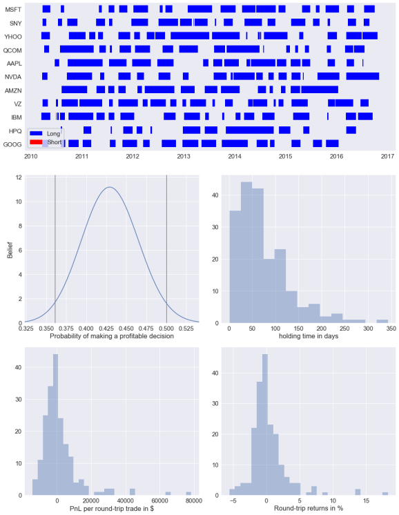
Above I found the round-trip statistics for my strategy during the backtest (that is, how trades tended to perform). We can see how many trades were conducted, how long the strategy tended to be in the market, how profitable trades tended to be, extreme statistic (largest winning trade, largest losing trade, max duration of a trade, etc.), how profitable certain symbols were, and many other useful metrics, along with graphics. This is much more digestable than the backtrader Analyzers default outputs.
Unfortunately, with Yahoo! Finance’s recent changes breaking pandas-datareader, PyFolio is not very stable right now and won’t be until pandas-datareader is updated. This is unfortunate, and reveals a flaw in PyFolio‘s design; using alternative data sources (both online and offline) for the data provided in their tear sheet functions should be better supported. While I was able to get the code below to work, this require some hacks and rolling back of packages. I cannot guarantee the code will work for you at this time. Additionally, some of the graphics PyFolio wants to create (such as comparing the performance of the strategy to SPY) don’t work since PyFolio can’t fetch the data.
Anyway, what does PyFolio include in its “full” tear sheet? We have some of the usual performance metrics, along with some more exotic ones, such as:
- The Calmar ratio, a risk-adjusted performance metric comparing compound rate of returns to the maximum drawdown.
- The Omega ratio, a newer and more exotic performance metric that effectively compares the gains of an investment to its losses, relative to some target.
- Skew, which describes the shape of the distribution of returns; a positive skew indicates a longer tail for gains (that is, more “extreme” values for gains), a negative value a longer tail for losses, and a skew of 0 indicates a symmetric distribution of returns around their mean.
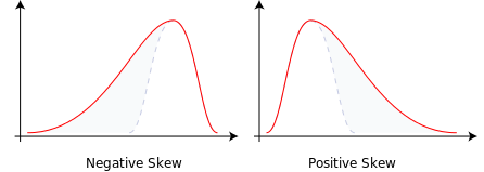
An illustration of positive and negative skewness provided by Wikipedia. - Kurtosis, another descriptor of the shape of the distribution of returns; a kurtosis larger than 3 indicates that the distribution is more “spread out” than the Normal distribution and indicates that extreme values in returns are more common, while a kurtosis smaller than 3 indicates that returns are more concentrated than if they were Normally distributed. Sometimes people describe “excess kurtosis”, where the Normal distribution has an excess kurtosis of zero and other distributions have an excess kurtosis above or below zero (so take kurtosis and subtract 3).
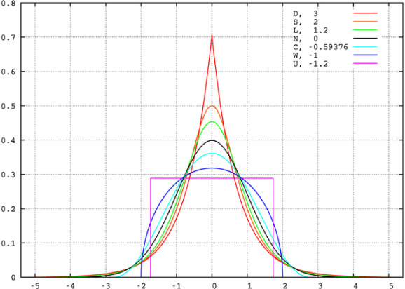
Visualization of distributions with different kurtosis, provided by Wikipedia. Notice that the legend displays excess kurtosis, or kurtosis minus three. All of these distributions have mean zero and variance one, yet still can be more or less spread out around the center than the Normal distribution. - Tail ratio, which is the ratio between the 95th percentile of returns and the absolute value of the 5th percentile of returns (so a tail ratio of 0.5 would imply that losses were twice as bad as winnings); the larger this number is, the better extreme winnings are compared to extreme losses.
- If the profit ratio is total profits divided by total losses, then the common sense ratio is the profit ratio multiplied with the tail ratio.
- Information ratio, which is the excess return of the strategy relative to a benchmark index divided by the standard deviation of the difference in returns between the strategy and the benchmark. (Here, since I had to use a constant benchmark return representing the risk-free rate, this number is not working as it should; again, you can send your gratitude to Verizon and tell them you approve of what they’ve done with Yahoo! Finance.)
- Alpha, which is performance relative to risk or some benchmark. Positive alpha is good, negative alpha is bad. (Again, not working right now.)
- Beta, the volatility of an asset relative to its benchmark. A beta less than one is good (less volatile than the market), while a beta greater than one is bad (more volatile than the market). (Not currently working.)
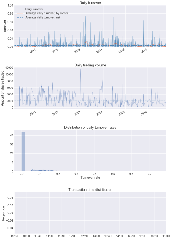
- Turnover, or how much of the account is sold in trades; a high turnover rate means higher commissions.
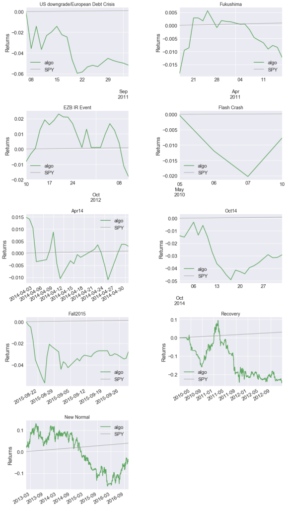
- Reaction to stress events, such as the Fukushima disaster, the 2010 Flash Crash, and others.
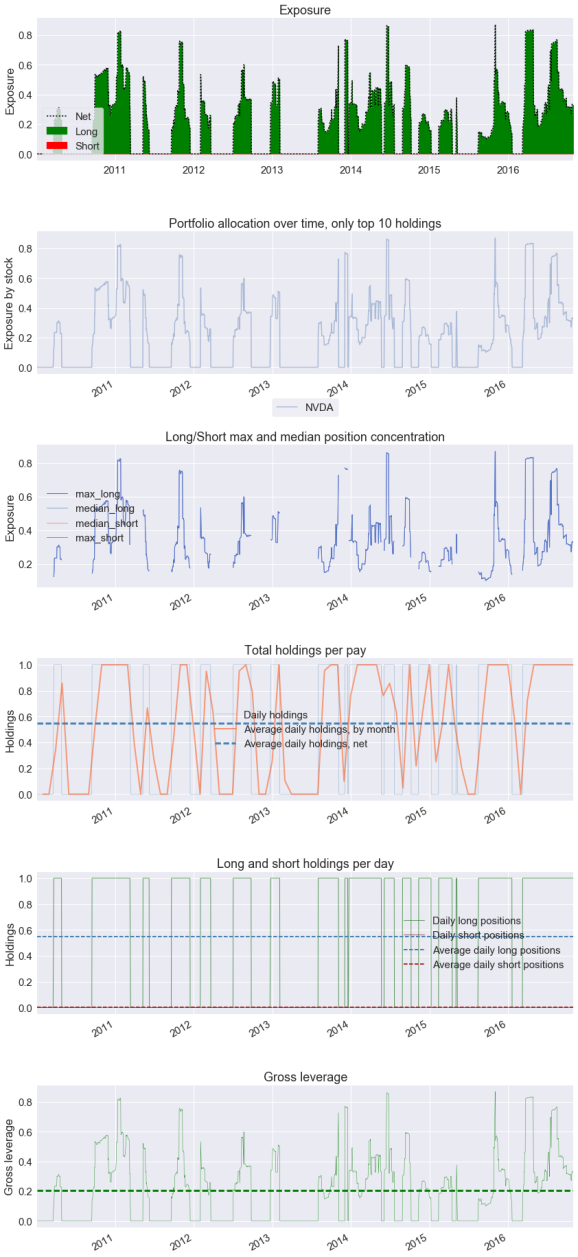
For some reason, create_full_tear_sheet() does not seem to be aware of other symbols being traded than Nvidia (NVDA). I have no idea why.
I create the full tear sheet below.
len(returns.index)
1720
benchmark_rets = pd.Series([0.00004] * len(returns.index), index=returns.index) # Risk-free rate, we need to
# set this ourselves otherwise
# PyFolio will try to fetch from
# Yahoo! Finance which is now garbage
# NOTE: Thanks to Yahoo! Finance giving the finger to their users (thanks Verizon, we love you too),
# PyFolio is unstable and will be until updates are made to pandas-datareader, so there may be issues
# using it
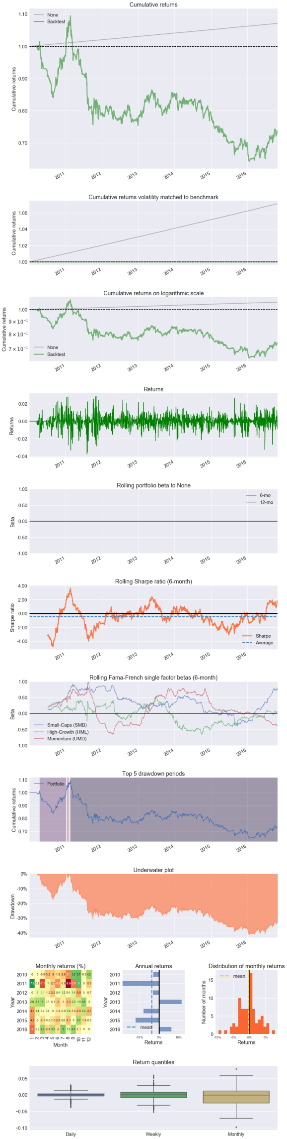
pf.create_full_tear_sheet(returns, positions, transactions, benchmark_rets=benchmark_rets)
Entire data start date: 2010-01-04
Entire data end date: 2016-10-31
Backtest Months: 81
| Performance statistics | Backtest |
|---|---|
| annual_return | -0.04 |
| cum_returns_final | -0.26 |
| annual_volatility | 0.11 |
| sharpe_ratio | -0.34 |
| calmar_ratio | -0.11 |
| stability_of_timeseries | 0.72 |
| max_drawdown | -0.41 |
| omega_ratio | 0.94 |
| sortino_ratio | -0.46 |
| skew | -0.27 |
| kurtosis | 3.14 |
| tail_ratio | 0.95 |
| common_sense_ratio | 0.90 |
| gross_leverage | 0.20 |
| information_ratio | -0.03 |
| alpha | nan |
| beta | nan |
| Worst drawdown periods | net drawdown in % | peak date | valley date | recovery date | duration |
|---|---|---|---|---|---|
| 0 | 41.30 | 2011-02-17 | 2016-01-20 | NaT | NaN |
| 1 | 17.11 | 2010-04-15 | 2010-08-30 | 2011-01-06 | 191 |
| 2 | 2.77 | 2011-01-14 | 2011-01-21 | 2011-01-27 | 10 |
| 3 | 2.74 | 2011-01-27 | 2011-01-28 | 2011-02-04 | 7 |
| 4 | 1.39 | 2011-02-04 | 2011-02-10 | 2011-02-17 | 10 |
[-0.014 -0.032]
| Stress Events | mean | min | max |
|---|---|---|---|
| US downgrade/European Debt Crisis | -0.25% | -3.53% | 2.24% |
| Fukushima | -0.05% | -1.83% | 1.15% |
| EZB IR Event | -0.08% | -1.52% | 1.22% |
| Flash Crash | -0.19% | -1.16% | 1.28% |
| Apr14 | 0.02% | -1.39% | 1.49% |
| Oct14 | -0.13% | -1.40% | 0.81% |
| Fall2015 | -0.08% | -1.85% | 2.62% |
| Recovery | -0.03% | -3.78% | 2.91% |
| New Normal | -0.00% | -3.23% | 2.62% |
| Top 10 long positions of all time | max |
|---|---|
| NVDA | 86.99% |
| Top 10 short positions of all time | max |
|---|
| Top 10 positions of all time | max |
|---|---|
| NVDA | 86.99% |
| All positions ever held | max |
|---|---|
| NVDA | 86.99% |
/home/curtis/anaconda3/lib/python3.6/site-packages/statsmodels/nonparametric/kdetools.py:20: VisibleDeprecationWarning: using a non-integer number instead of an integer will result in an error in the future
  y = X[:m/2+1] + np.r_[0,X[m/2+1:],0]*1j
Optimizing with Different Metrics
Instead of optimizing with respect to returns, we may want to optimize with respect to a risk-adjusted metric, such as the Sharpe ratio. We can investigate the results of using different metrics for optimization with walk-forward analysis.
In walk-forward analysis we might add an additional metric to our arsenal, the walk-forward efficiency ratio (WFER). This ratio gives a sens of our system’s out-of-sample performance. If we were optimizing with respect to returns, we’d divide out-of-sample returns by the returns obtained by the optimized strategy. If this is greater than 1, our out-of-sample returns were higher than optimized returns, while if this is less than 1, out-of-sample returns are less than optimized returns. This can be applied to any metric we use for optimization, and gives a sense for how much our strategy tends to overfit. A low WFER suggests a high propensity to overfit. (Unfortunately, my code for WFER doesn’t seem to be correct right now.)
Below I create a function to automate the walk-forward analysis process. You pass the function a Cerebro object with everything added to it except the strategy and the data; these are passed as arguments to the function and will be handled by it. (You can only work with one strategy at a time.) All analyzers are combined together into one dictionary at the end of one iteration, and all of these dictionaries are returned in a list. If the dictionaries are all flat, this list can easily be converted to a pandas DataFrame.
def wfa(cerebro, strategy, opt_param, split, datafeeds, analyzer_max, var_maximize,
        opt_p_vals, opt_p_vals_args={}, params={}, minimize=False):
    """Perform a walk-forward analysis

    args:
        cerebro: A Cerebro object, with everything added except the strategy and data feeds; that is, all
            analyzers, sizers, starting balance, etc. needed have been added
        strategy: A Strategy object for optimizing
        params: A dict that contains all parameters to be set for the Strategy except the parameter to be
            optimized
        split: Defines the splitting of the data into training and test sets, perhaps created by
            TimeSeriesSplit.split()
        datafeeds: A dict containing pandas DataFrames that are the data feeds to be added to Cerebro
            objects and used by the strategy; keys are the names of the strategies
        analyzer_max: A string denoting the name of the analyzer with the statistic to maximize
        var_maximize: A string denoting the variable to maximize (perhaps the key of a dict)
        opt_param: A string: the parameter of the strategy being optimized
        opt_p_vals: This can be either a list or function; if a function, it must return a list, and the
            list will contain possible values that opt_param will take in optimization; if a list, it already
            contains these values
        opt_p_vals_args: A dict of parameters to pass to opt_p_vals; ignored if opt_p_vals is not a function
        minimize: A boolean that if True will minimize the parameter rather than maximize

    return:
        A list of dicts that contain data for the walk-forward analysis, including the relevant
        analyzer's data, the value of the optimized statistic on the training set, start and end dates for
        the test set, and the walk forward efficiency ratio (WFER)
    """

    usr_opt_p_vals = opt_p_vals
    walk_forward_results = list()
    for train, test in split:
        trainer, tester = deepcopy(cerebro), deepcopy(cerebro)

        if callable(usr_opt_p_vals):
            opt_p_vals = usr_opt_p_vals(**opt_p_vals_args)

        # TRAINING
        trainer.optstrategy(strategy, **params, **{opt_param: opt_p_vals})
        for s, df in datafeeds.items():
            data = bt.feeds.PandasData(dataname=df.iloc[train], name=s)
            trainer.adddata(data)
        res = trainer.run()
        res_df = DataFrame({getattr(r[0].params, opt_param): dict(getattr(r[0].analyzers,
                                                                          analyzer_max).get_analysis()) for r in res}
                       ).T.loc[:, var_maximize].sort_values(ascending=minimize)
        opt_res, opt_val = res_df.index[0], res_df[0]

        # TESTING
        tester.addstrategy(strategy, **params, **{opt_param: opt_res})
        for s, df in datafeeds.items():
            data = bt.feeds.PandasData(dataname=df.iloc[test], name=s)
            tester.adddata(data)
        res = tester.run()
        res_dict = dict(getattr(res[0].analyzers, analyzer_max).get_analysis())
        res_dict["train_" + var_maximize] = opt_val
        res_dict[opt_param] = opt_res
        s0 = [*datafeeds.keys()][0]
        res_dict["start_date"] = datafeeds[s0].iloc[test[0]].name
        res_dict["end_date"] = datafeeds[s0].iloc[test[-1]].name
        test_val = getattr(res[0].analyzers, analyzer_max).get_analysis()[var_maximize]
        try:
            res_dict["WFER"] = test_val / opt_val
        except:
            res_dict["WFER"] = np.nan
        for anlz in res[0].analyzers:
            res_dict.update(dict(anlz.get_analysis()))

        walk_forward_results.append(res_dict)

    return walk_forward_results
The function can be given a list of possible choices of parameters to optimize over, but can also accept a function that generates this list (perhaps you are choosing possible parameter values randomly). I create a generator function below, that will be used in the walk-forward analysis.
def random_fs_list():
    """Generate random combinations of fast and slow window lengths to test"""
    windowset = set()    # Use a set to avoid duplicates
    while len(windowset) < 40:
        f = random.randint(1, 10) * 5
        s = random.randint(1, 10) * 10
        if f > s:    # Cannot have the fast moving average have a longer window than the slow, so swap
            f, s = s, f
        elif f == s:    # Cannot be equal, so do nothing, discarding results
            continue
        windowset.add((f, s))

    return list(windowset)
Now let’s get the walk-forward analysis results when optimizing with respect to the Sharpe ratio.
walkorebro = bt.Cerebro(stdstats=False, maxcpus=1)

walkorebro.broker.setcash(1000000)
walkorebro.broker.setcommission(0.02)
walkorebro.addanalyzer(btanal.SharpeRatio_A)
walkorebro.addanalyzer(btanal.Returns)
walkorebro.addanalyzer(AcctStats)
walkorebro.addsizer(PropSizer)

tscv = TimeSeriesSplitImproved(10)
split = tscv.split(datafeeds["AAPL"], fixed_length=True, train_splits=2)


%time wfa_sharpe_res = wfa(walkorebro, SMAC, opt_param="optim_fs", params={"optim": True}, \
                           split=split, datafeeds=datafeeds, analyzer_max="sharperatio_a", \
                           var_maximize="sharperatio", opt_p_vals=random_fs_list)

CPU times: user 2h 7min 13s, sys: 2.55 s, total: 2h 7min 15s
Wall time: 2h 8min 1s


DataFrame(wfa_sharpe_res)
| WFER | end | end_date | growth | optim_fs | ravg | return | rnorm | rnorm100 | rtot | sharperatio | start | start_date | train_sharperatio | |
|---|---|---|---|---|---|---|---|---|---|---|---|---|---|---|
| 0 | NaN | 953091.50 | 2011-11-14 | -46908.50 | (45, 70) | -0.000306 | 0.953091 | -0.074217 | -7.421736 | -0.048044 | NaN | 1000000 | 2011-04-05 | 3.377805 |
| 1 | 1.274973 | 892315.80 | 2012-06-28 | -107684.20 | (10, 30) | -0.000726 | 0.892316 | -0.167129 | -16.712927 | -0.113935 | -1.237580 | 1000000 | 2011-11-15 | -0.970672 |
| 2 | 1.195509 | 1007443.84 | 2013-02-13 | 7443.84 | (15, 90) | 0.000047 | 1.007444 | 0.011975 | 1.197496 | 0.007416 | -0.527568 | 1000000 | 2012-06-29 | -0.441292 |
| 3 | NaN | 1008344.50 | 2013-09-26 | 8344.50 | (15, 70) | 0.000053 | 1.008345 | 0.013427 | 1.342750 | 0.008310 | NaN | 1000000 | 2013-02-14 | 0.480783 |
| 4 | -3.030306 | 991597.32 | 2014-05-12 | -8402.68 | (40, 70) | -0.000054 | 0.991597 | -0.013453 | -1.345278 | -0.008438 | -3.380193 | 1000000 | 2013-09-27 | 1.115463 |
| 5 | NaN | 960946.16 | 2014-12-22 | -39053.84 | (20, 70) | -0.000254 | 0.960946 | -0.061941 | -6.194062 | -0.039837 | NaN | 1000000 | 2014-05-13 | 0.636099 |
| 6 | -4.286899 | 966705.62 | 2015-08-06 | -33294.38 | (20, 80) | -0.000216 | 0.966706 | -0.052900 | -5.289996 | -0.033861 | -1.600702 | 1000000 | 2014-12-23 | 0.373394 |
| 7 | 0.293385 | 1011624.06 | 2016-03-21 | 11624.06 | (25, 90) | 0.000074 | 1.011624 | 0.018723 | 1.872324 | 0.011557 | -0.623374 | 1000000 | 2015-08-07 | -2.124761 |
| 8 | NaN | 994889.98 | 2016-10-31 | -5110.02 | (40, 100) | -0.000033 | 0.994890 | -0.008189 | -0.818938 | -0.005123 | NaN | 1000000 | 2016-03-22 | -0.462381 |
Returns are arguable better here than when I optimized with respect to just returns since a catastrophically bad strategy was avoided, but I’m not convinced we’re doing any better.
Let’s try with the Sortino ratio now. I have a few reasons for favoring the Sortino ratio as a risk measure:
- The Sortino ratio uses the standard deviation of losses, which we might call “bad risk”.
- Measures reliant on “standard deviaton” implicitly assume Normally distributed returns or that returns are well-behaved in some sense, but if returns follow, say, a power law, where “extreme events are common”, the standard deviation is not a good measure for risk. Theoretically, the standard deviation may not be well-defined. Since losses are truncated, though (meaning that there is a maximum loss that can be attained), standard deviation for losses should exist theoretically, so we can avoid some these issues. Furthermore, extreme events should make this standard deviation larger rather than smaller (since standard deviation is sensitive to outliers), which makes the overall ratio smaller and thus more conservative in the presence of outlier losses.
Let’s see the results when using the Sortino ratio in place of the Sharpe ratio.
walkorebro.addanalyzer(SortinoRatio)

split = tscv.split(datafeeds["AAPL"], fixed_length=True, train_splits=2)


%time wfa_sortino_res = wfa(walkorebro, SMAC, opt_param="optim_fs", params={"optim": True}, \
                            split=split, datafeeds=datafeeds, analyzer_max="sortinoratio", \
                            var_maximize="sortinoratio", opt_p_vals=random_fs_list)

/home/curtis/anaconda3/lib/python3.6/site-packages/ipykernel/__main__.py:50: RuntimeWarning: invalid value encountered in log


CPU times: user 2h 7min 33s, sys: 9.39 s, total: 2h 7min 43s
Wall time: 2h 8min 38s


DataFrame(wfa_sortino_res)
| WFER | end | end_date | growth | optim_fs | ravg | return | rnorm | rnorm100 | rtot | sharperatio | sortinoratio | start | start_date | train_sortinoratio | |
|---|---|---|---|---|---|---|---|---|---|---|---|---|---|---|---|
| 0 | -0.285042 | 988750.90 | 2011-11-14 | -11249.10 | (45, 90) | -0.000072 | 0.988751 | -0.017994 | -1.799434 | -0.011313 | NaN | -0.033131 | 1000000 | 2011-04-05 | 0.116231 |
| 1 | -6.620045 | 1007201.00 | 2012-06-28 | 7201.00 | (50, 100) | 0.000046 | 1.007201 | 0.011583 | 1.158345 | 0.007175 | -1.777392 | 0.097353 | 1000000 | 2011-11-15 | -0.014706 |
| 2 | 3.543051 | 1007443.84 | 2013-02-13 | 7443.84 | (15, 90) | 0.000047 | 1.007444 | 0.011975 | 1.197496 | 0.007416 | -0.527568 | 0.038794 | 1000000 | 2012-06-29 | 0.010949 |
| 3 | 0.861968 | 1008344.50 | 2013-09-26 | 8344.50 | (15, 70) | 0.000053 | 1.008345 | 0.013427 | 1.342750 | 0.008310 | NaN | 0.042481 | 1000000 | 2013-02-14 | 0.049283 |
| 4 | -0.051777 | 998959.50 | 2014-05-12 | -1040.50 | (35, 70) | -0.000007 | 0.998960 | -0.001670 | -0.166958 | -0.001041 | -20.221528 | -0.006508 | 1000000 | 2013-09-27 | 0.125685 |
| 5 | -2.029468 | 972178.20 | 2014-12-22 | -27821.80 | (30, 80) | -0.000180 | 0.972178 | -0.044279 | -4.427936 | -0.028216 | NaN | -0.157309 | 1000000 | 2014-05-13 | 0.077512 |
| 6 | -4.718336 | 976411.72 | 2015-08-06 | -23588.28 | (45, 80) | -0.000152 | 0.976412 | -0.037590 | -3.759040 | -0.023871 | -1.847879 | -0.130495 | 1000000 | 2014-12-23 | 0.027657 |
| 7 | -8.761974 | 1012292.72 | 2016-03-21 | 12292.72 | (30, 90) | 0.000078 | 1.012293 | 0.019804 | 1.980425 | 0.012218 | -0.441576 | 0.176737 | 1000000 | 2015-08-07 | -0.020171 |
| 8 | NaN | 1000000.00 | 2016-10-31 | 0.00 | (20, 100) | 0.000000 | 1.000000 | 0.000000 | 0.000000 | 0.000000 | NaN | NaN | 1000000 | 2016-03-22 | -0.017480 |
This is better, but far from impressive. These analyses reinforce my opinion that the SMAC strategy does not work for the symbols I’ve considered. I would be better off abandoning this line of investigatioin and looking elsewhere.
Conclusion, and Thoughts On Blogging
Up to this point, I have been interested mostly in investigating backtesting technology. I wanted to see which packages would allow me to do what I feel I should be able to do with a backtesting system. If I were to move on from this point, I would be looking at identifying different trading systems, not just “how to optimize”, “how to do a walk-forward analysis”, or “how to get the metrics I want from a backtest.”
Now to drift off-topic.
I’ve enjoyed blogging on these topics, but I’ve run into a problem. See, I’m still a graduate student, hoping to get a PhD. I started this blog as a hobby, but these days I have been investing a lot of time into writing these blog posts, which have been technically challenging for me. I spend days researching, writing, and debugging code. I write new blog posts, investing a lot of time in them. I personally grow a lot. Then I look at my website’s stats, and see that despite all the new content I write, perhaps 90% of all the traffic to this blog goes to three blog posts. Despite the fact that I believe I’ve written content that is more interesting than these posts, that content gets hardly any traffic.
I recently read a response to a Quora question, written by Prof. Ben Y. Zhao at the University of Chicago that rattled me. In his answer, Prof. Zhao says:
I might also add that “gaining knowledge in many areas/fields” is likely to be detrimental to getting a PhD. Enjoying many different fields generally translates into a lack of focus in the context of a PhD program, and you’re likely to spend more time marveling over papers from a wide range of topics rather than focusing and digging deep to produce your own research contributions.
As a person who has a lot of interests, I’m bothered by this comment. A lot.
This blog has lead to some book contracts for me. I have one video course introducing NumPy and pandas coming out in a few days, published by Packt Publishing (I will write a post about it not long after it’s out). This was a massive time commitment on my part, more than I thought it would be (I am always significantly underestimating how much time projects will take). When I initially told one of my former professors at the University of Utah that I had been offered a contract to create some video courses, he became upset, almost yelling at me, criticizing me for not “guarding your time.” (My professor directed me to another member of the deparment who had written books in hope that he would disuade me by telling me what the process was like; instead he recommended that I leverage the book deal I got into other book deals, which is the opposite of what my professor intended.)
I couldn’t resist the allure of being published so I agreed to the deal and signed the contracts, but since then, I’ve begun wishing I listened to my professor’s advice. I have two qualifying exams coming up in August, and I don’t feel like I have done nearly enough to prepare for them, partly due to the book deal, and partly due to the time I spend writing blog posts (and I also read too much). Furthermore, I have committed to three more volumes and I don’t want to break a contract; I agreed to do something and I intend to see it to the end. Meanwhile, other publishers have offered me publishing deals and I’m greatly pained whenever I say “no”; I like creating content like this, I like the idea of having a portfolio of published works providing a source of prestige and passive income (and with my rent having increased by over \$100 in two years when I could barely afford it in the first place, I could really use that extra income right now).
Long story short, time is an even scarcer commodity now than it used to be for me. I’m worried about my academic success if I keep burning time like this. It also doesn’t seem like any of my new content “sticks” (it doesn’t bump up what you might call my “latent” viewership rate).
Thus, I’m planning on this being my last “long-form” article for some time. I’m slightly heartbroken to say this. I would love to write more articles about agent-based modelling (particularly the Santa Fe Artificial Stock Market or developing a model for the evolution of party systems in republics), finance and algorithmic trading, statistical models for voting in legislatures (like DW-NOMINATE), and many others. I have notebooks filled with article ideas. I cannot afford the time, though.
I may post occasionally, perhaps with a few code snippets or to announce my video courses. I won’t try to keep a regular schedule, though, and I won’t be writing specifically for the site (that is, something in my studies prompted the topic).
For those reading this article, I would still love to hear your comments on algorithmic trading and if there are areas you are curious about. I’d likely put those into my notebook of ideas to investigate and perhaps I will look into them. I’ve learned a lot maintaining this website and I hope eventually to return to writing weekly long-form articles on topics I’m interested in again someday. Algorithmic trading still intreagues me and I want to play with it from time to time.
Thank you all for reading. When I started blogging, I was hoping to get maybe 70 views in a week. I never imagined I’d be getting at least 400 every day (usually around 500 or 600, sometimes 1,000 on the day of a new post). This took me a lot farther than I thought I would go, and it’s been a great trip in the meantime.
I have created a video course that Packt Publishing will be publishing later this month, entitled Unpacking NumPy and Pandas, the first volume in a four-volume set of video courses entitled, Taming Data with Python; Excelling as a Data Analyst. This course covers the basics of setting up a Python environment for data analysis with Anaconda, using Jupyter notebooks, and using NumPy and pandas. If you are starting out using Python for data analysis or know someone who is, please consider buying my course or at least spreading the word about it. You can buy the course directly or purchase a subscription to Mapt and watch it there (when it becomes available).
If you like my blog and would like to support it, spread the word (if not get a copy yourself)! Also, stay tuned for future courses I publish with Packt at the Video Courses section of my site.

R-bloggers.com offers daily e-mail updates about R news and tutorials about learning R and many other topics. Click here if you're looking to post or find an R/data-science job.
Want to share your content on R-bloggers? click here if you have a blog, or here if you don't.