When query execution performance analysis is to be done, there are many ways to find which queries might cause any unwanted load or cause stall on the server.

By encouraging DBA community to start practicing the advantage or R Language and world of data science, I have created a demo to show, how statistics on numerous queries can be stored for later analysis. And this demo has unsupervised (or undirected) method for grouping similar query statistics (or queries) to easier track and find where and which queries might be potential system stoppers.

Before we run some queries to generate the running statistics for these queries, we clean the cache and prepare the table for storing statistics from sys.dm_exec_query_stats.

-- drop statistics table
DROP TABLE IF EXISTS  query_stats_LOG_2;
DROP PROCEDURE IF EXISTS AbtQry;
DROP PROCEDURE IF EXISTS SalQry;
DROP PROCEDURE IF EXISTS PrsQry;
DROP PROCEDURE IF EXISTS OrdQry;
DROP PROCEDURE IF EXISTS PurQry;
GO

-- Clean all the stuff only for the selected db
DECLARE @dbid INTEGER
SELECT @dbid = [dbid] 
FROM master..sysdatabases 
WHERE name = 'WideWorldImportersDW'
DBCC FLUSHPROCINDB (@dbid);
GO

-- for better sample, check that you have Query store turned off
ALTER DATABASE WideWorldImportersDW SET  QUERY_STORE = OFF;
GO

We generate some fake data:

USE WideWorldImportersDW;
GO

-- CREATE Procedures 

CREATE PROCEDURE AbtQry
(@AMNT AS INTEGER) 
AS

-- an arbitrary query
SELECT 
  cu.[Customer Key] AS CustomerKey
  ,cu.Customer
  ,ci.[City Key] AS CityKey
  ,ci.City
  ,ci.[State Province] AS StateProvince
  ,ci.[Sales Territory] AS SalesTeritory
  ,d.Date
  ,d.[Calendar Month Label] AS CalendarMonth
  ,s.[Stock Item Key] AS StockItemKey
  ,s.[Stock Item] AS Product
  ,s.Color
  ,e.[Employee Key] AS EmployeeKey
  ,e.Employee
  ,f.Quantity
  ,f.[Total Excluding Tax] AS TotalAmount
  ,f.Profit
 
FROM Fact.Sale AS f
  INNER JOIN Dimension.Customer AS cu
    ON f.[Customer Key] = cu.[Customer Key]
  INNER JOIN Dimension.City AS ci
    ON f.[City Key] = ci.[City Key]
  INNER JOIN Dimension.[Stock Item] AS s
    ON f.[Stock Item Key] = s.[Stock Item Key]
  INNER JOIN Dimension.Employee AS e
    ON f.[Salesperson Key] = e.[Employee Key]
  INNER JOIN Dimension.Date AS d
    ON f.[Delivery Date Key] = d.Date
WHERE
    f.[Total Excluding Tax] BETWEEN 10 AND @AMNT;
GO

CREATE PROCEDURE SalQry
(@Q1 AS INTEGER
,@Q2 AS INTEGER)

AS
-- FactSales Query
SELECT * FROM Fact.Sale
WHERE
    Quantity BETWEEN @Q1 AND @Q2;
GO

CREATE PROCEDURE PrsQry
(@CID AS INTEGER )
AS

-- Person Query
SELECT * 
    FROM [Dimension].[Customer]
    WHERE [Buying Group] <> 'Tailspin Toys' 
    /* OR [WWI Customer ID] > 500 */
    AND [WWI Customer ID] BETWEEN 400 AND  @CID
ORDER BY [Customer],[Bill To Customer];
GO


CREATE PROCEDURE OrdQry
(@CK AS INTEGER)
AS

-- FactSales Query
SELECT 
    * 
    FROM [Fact].[Order] AS o
    INNER JOIN [Fact].[Purchase] AS p 
    ON o.[Order Key] = p.[WWI Purchase Order ID]
WHERE
    o.[Customer Key] = @CK;
GO

CREATE PROCEDURE PurQry
(@Date AS SMALLDATETIME)
AS

-- FactPurchase Query
SELECT *
    FROM [Fact].[Purchase]
        WHERE
        [Date Key] = @Date;
    --[Date KEy] = '2015/01/01'
GO

Now we run procedures couple of times:

DECLARE @ra DECIMAL(10,2)
SET @ra = RAND()
SELECT CAST(@ra*10 AS INT)

IF @ra  < 0.3333
    BEGIN
       -- SELECT 'RAND < 0.333', @ra
       DECLARE @AMNT_i1 INT = 100*CAST(@ra*10 AS INT)
       EXECUTE AbtQry @AMNT = @AMNT_i1
       EXECUTE PurQry @DAte = '2015/10/01'
       EXECUTE PrsQry @CID = 480
       EXECUTE OrdQry @CK = 0
       DECLARE @Q1_i1 INT = 1*CAST(@ra*10 AS INT)
       DECLARE @Q2_i1 INT = 20*CAST(@ra*10 AS INT)
       EXECUTE SalQry @Q1 = @Q1_i1, @Q2 = @Q2_i1

    END
ELSE 
    IF @ra  > 0.3333 AND @ra < 0.6667
    BEGIN
        -- SELECT 'RAND > 0.333 | < 0.6667', @ra
        DECLARE @AMNT_i2 INT = 500*CAST(@ra*10 AS INT)
        EXECUTE AbtQry @AMNT = @AMNT_i2
        EXECUTE PurQry @DAte = '2016/04/29'
        EXECUTE PrsQry @CID = 500
        EXECUTE OrdQry @CK = 207
        DECLARE @Q1_i2 INT = 2*CAST(@ra*10 AS INT)
        DECLARE @Q2_i2 INT = 10*CAST(@ra*10 AS INT)
        EXECUTE SalQry @Q1 = @Q1_i2, @Q2 = @Q2_i2

    END
ELSE
    BEGIN
        -- SELECT 'RAND > 0.6667', @ra
        DECLARE @AMNT_i3 INT = 800*CAST(@ra*10 AS INT)
        EXECUTE AbtQry @AMNT = @AMNT_i3
        EXECUTE PurQry @DAte = '2015/08/13'
        EXECUTE PrsQry @CID = 520
        EXECUTE OrdQry @CK = 5
        DECLARE @Q2_i3 INT = 60*CAST(@ra*10 AS INT)
        EXECUTE SalQry @Q1 = 25, @Q2 = @Q2_i3
    END
GO 10

And with this data, we proceed to run the logging T-SQL (query source).

SELECT
    (total_logical_reads + total_logical_writes) AS total_logical_io
    ,(total_logical_reads / execution_count) AS avg_logical_reads
    ,(total_logical_writes / execution_count) AS avg_logical_writes
    ,(total_physical_reads / execution_count) AS avg_phys_reads
    ,substring(st.text,(qs.statement_start_offset / 2) + 1,  
      ((CASE qs.statement_end_offset WHEN - 1 THEN datalength(st.text) 
   qs.statement_end_offset END  - qs.statement_start_offset) / 2) + 1) 
AS statement_text
    ,*
INTO query_stats_LOG_2
FROM
        sys.dm_exec_query_stats AS qs
    CROSS APPLY sys.dm_exec_sql_text(qs.sql_handle) AS st
ORDER BY total_logical_io DESC

Now that we have gathered some test data, we can proceed to do clustering analysis.

Since I don’t know how many clusters can there be, and I can imagine, a  DBA would also be pretty much clueless, I will explore number of clusters. Following R code:

library(RODBC)
myconn <-odbcDriverConnect("driver={SQL Server};Server=SICN-KASTRUN;
database=WideWorldImportersDW;trusted_connection=true")

query.data <- sqlQuery(myconn, "
                     SELECT 
                                 [total_logical_io]
                      ,[avg_logical_reads]
                      ,[avg_phys_reads]
                      ,execution_count
                      ,[total_physical_reads]
                      ,[total_elapsed_time]
                      ,total_dop
                      ,[text]
                      ,CASE WHEN LEFT([text],70) LIKE '%AbtQry%' THEN 'AbtQry'
                       WHEN LEFT([text],70) LIKE '%OrdQry%' THEN 'OrdQry'
                       WHEN LEFT([text],70) LIKE '%PrsQry%' THEN 'PrsQry'
                       WHEN LEFT([text],70) LIKE '%SalQry%' THEN 'SalQry'
                       WHEN LEFT([text],70) LIKE '%PurQry%' THEN 'PurQry'
                       HEN LEFT([text],70) LIKE '%@BatchID%' THEN 'System'
                                  ELSE 'Others' END AS label_graph 
                      FROM query_stats_LOG_2")

close(myconn) 
library(cluster)

#qd <- query.data[,c(1,2,3,5,6)]
qd <- query.data[,c(1,2,6)]

## hierarchical clustering
qd.use <- query.data[,c(1,2,6)]
medians <- apply(qd.use,2,median)
#mads <- apply(qd.use,2,mad)
qd.use <- scale(qd.use,center=medians) #,scale=mads)

#calculate distances
query.dist <- dist(qd.use)

# hierarchical clustering
query.hclust <- hclust(query.dist)

# plotting solution
op <- par(bg = "lightblue")
plot(query.hclust,labels=query.data$label_graph,
main='Query Hierarchical Clustering', ylab = 'Distance', 
xlab = ' ', hang = -1, sub = "" )
# in addition to circle queries within cluster
rect.hclust(query.hclust, k=3, border="DarkRed")        

And produces the following plot:

Graph itself is self explanatory and based on the gathered statistics and queries executed against the system, you receive the groups of queries where your DBA can easily and fast track down what might be causing some issues. I added some labels to the query for the graph to look neater, but it is up to you.

I have also changed the type to “triangle” to get the following plot:

And both show same information.

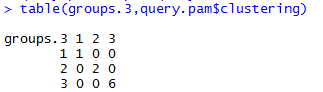
So the R code said that, there are three clusters generating And I used medians to generate data around it. In addition I have also tested the result with Partitioning around medoids (which is opposite to hierarchical clustering) and the results from both techniques yield clean clusters.

Also, the data sample is relatively small, but you are very welcome to test this idea into your environment. Just easy with freeproccache and flushprocindb commands!

This blog post was meant as a teaser,  to gather opinion from the readers. Couple of more additional approaches will be part of two articles, that I am currently working on.

As always, code is available at the Github.

Happy SQLinRg!