In my previous blog post, I was focusing on data manipulation tasks with RevoScaleR Package in comparison to other data manipulation packages and at the end conclusions were obvious; RevoScaleR can not (without the help of dplyrXdf) do piping (or chaining) and storing temporary results take time and on top of that, data manipulation can be done easier (cleaner and faster) with dplyr package or data.table package. Another conclusion was, that you should do (as much as possible) all the data manipulation tasks within your client, so you diminish the value of the data sent to computation environment.

In this post, I will do a simple performance comparison between  kmeans clustering function  available in default stats package and RevoScaleR rxKmeans function for clustering.

Data will be loaded from WideWorldImportersDW.

library(RODBC)
library(RevoScaleR)
library(ggplot2)
library(dplyr)

myconn <-odbcDriverConnect("driver={SQL Server};Server=T-KASTRUN;
database=WideWorldImportersDW;trusted_connection=true")

cust.data <- sqlQuery(myconn, "SELECT 
                      fs.[Sale Key] AS SalesID
                      ,fs.[City Key] AS CityKey
                      ,c.[City] AS City
                      ,c.[State Province] AS StateProvince
                      ,c.[Sales Territory] AS SalesTerritory
                      ,fs.[Customer Key] AS CustomerKey
                      ,fs.[Stock Item Key] AS StockItem
                      ,fs.[Quantity] AS Quantity
                      ,fs.[Total Including Tax] AS Total
                      ,fs.[Profit] AS Profit
                      
                      
                      FROM [Fact].[Sale] AS  fs
                      JOIN dimension.city AS c
                      ON c.[City Key] = fs.[City Key]
                      WHERE
                      fs.[customer key] <> 0 ")

close(myconn)

In essence, I will be using same dataset, and comparing same algorithm (Lloyd) with same variables (columns) taken with all parameters the same. So RevoScaleR rxKmeans with following columns:

rxSalesCluster <- rxKmeans(formula= ~SalesID + CityKey + CustomerKey + 
StockItem + Quantity, data =cust.data, numCluster=9,algorithm = "lloyd", 
outFile = "SalesCluster.xdf", outColName = "Cluster", overwrite = TRUE)

vs. kmeans example:

SalesCluster <- kmeans(cust.data[,c(1,2,6,7,8)], 9, nstart = 20, algorithm="Lloyd")

After running 50 iterations on both of the algorithms, measured two metrics. First one was elapsed computation time and second one was the ratio between the “between-cluster sum of squares” and “total within-cluster sum of squares”.

fit <- rxSalesCluster$betweenss/rxSalesCluster$totss

Graph of the performance over 50 iterations with both clustering functions.

The performance results are very much obvious, rxKmeans function from RevoScaleR package outperforms stats kmeans by almost 3-times, which is at given dataset (143K Rows and 5 variables) a pretty substantiate improvement due to parallel computation.

So in terms of elapsed computation time:

result %>%
  group_by(cl_met) %>%
  summarize(
    average_score = mean(et)
    ,variance = var(et)
    ,st_dev = sd(et)
  )

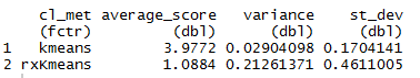
kmeans average computation time is little below 4 seconds and rxKmeans computation time is little over 1 second. Please keep in mind that additional computation is performed in this time for clusters fit but in terms of time difference, it remains the same. From graph and from variance/standard deviations, one can see that rxKmeans has higher deviations which results in spikes on graph and are results of parallelizing the data on file. Every 6th iteration there is additional workload / worker dedicated for additional computation.

But the biggest concern is the results itself. Over 50 iterations I stored also the computation of with-in and between cluster sum of squares calculations. And results are stunning.

result %>% 
  group_by(cl_met) %>%
  summarize(
             average_score = mean(fit)
            ,variance = var(fit)
            ,st_dev = sd(fit)
           )

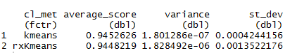
The difference between average calculation of the fit is absolutely so minor that it is worthless giving any special attention.

(mean(result[result$cl_met == 'kmeans',]$fit)*100 - mean(result[result$cl_met 
== 'rxKmeans',]$fit)*100)

is

0.04407133.

With rxKmeans you gain super good performances and the results are equal as to the default kmean clustering function.

Code is availble at GitHub.

Happy R-TSQLing!