Introduction

Although more than 20 years old, Market Basket Analysis (MBA) (or association rules mining) can still be a very useful technique to gain insights in large transactional data sets. The classical example is transactional data in a supermarket. For each customer we know what the individual products (items) are that he has put in his basket and bought. Other use cases for MBA could be web click data, log files, and even questionnaires.

With market basket analysis we can identify items that are frequently bought together. Usually the results of an MBA are presented in the form of rules. The rules can be as simple as {A ==> B}, when a customer buys item A then it is (very) likely that the customer buys item B. More complex rules are also possible {A, B ==> D, F}, when a customer buys items A and B then it is likely that he buys items D and F.

Soccer transactional data

To perform MBA you need of course data, but I don’t have real transactional data from a retailer that I can present here. So I am using soccer data instead From the Kaggle site you can download some soccer data, thanks to Hugo Mathien. The data contains around 25.000 matches from eleven European soccer leagues starting from season 2008/2009 until season 2015/2016. After some data wrangling I was able to generate a transactional data set suitable for market basket analysis. The data structure is very simple, some records are given in the figure below:

So we do not have customers but soccer players, and we do not have products but soccer clubs. In total, my soccer transactional data set contains around 18.000 records. Obviously, these records do not only include the multi-million transfers covered in the media, but also all the transfers of players nobody has ever heard of

Market basket results

In R you can use the arules package for MBA / association rules mining. Alternatively, when the order of the transactions is important, like my soccer transfers, you should use the arulesSequences package. After running the algorithm I got some interesting results. The figure below shows the most frequently occurring transfers between clubs:

So in this data set the most frequently occurring transfer is from Fiorentina to Genoa (12 transfers in total). I have published the entire table with the rules on RPubs, where you can look up the transfer activity of your favorite soccer club.

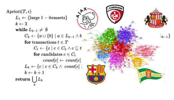
Network graph visualization

All the rules that we get from the association rules mining form a network graph. The individual soccer clubs are the nodes of the graph and each rule “from ==> to” is an edge of the graph. In R, network graphs can be visualized nicely by means of the visNetwork package. The network is shown in the picture below.

An interactive version can be found on RPubs. The different colors represent the different soccer leagues. There are eleven leagues in this data, there are more leagues in Europe, but in this data we see that the Polish league is quite isolated from the rest. Almost blended in each other are the German, Spanish, English and French leagues. Less connected are the Scottish and Portuguese leagues, but also in the big English Premier and German leagues you will find less connected clubs like Bournemouth, Reading or Arminia Bielefeld.

The size of a node in the above graph represents it’s betweenness centrality, it is an indicator of a node’s centrality in a network. It is equal to the number of shortest paths from all vertices to all others that pass through that node. In R betweenness measures can be calculated with the igraph package. The most central clubs in the transfers of players are Sporting CP, Lechia Gdansk, Sunderland, FC Porto and PSV Eindhoven.

Virtual Items

An old trick among marketeers is to use virtual items in a market basket analysis. Besides the ‘physical’ items that a customer has in his basket, a marketeer can add extra virtual items in the basket. These could be for example customer characteristic like age-class, sex, but also things like day of week, region etc. The transactional data with virtual items might look like:

If you run a MBA on the transactional data with virtual items, interesting rules might appear. For example:

• {Chocolate, Female ==> Eggs}
• {Chocolate, Male ==> Apples}
• {Beer, Friday, Male, Age[18:23] ==> sausages}.

Virtual items that I can add to my soccer transactional data are: age-class, four classes: 1: players younger than 25, 2: [25, 29), 3: [29, 33) and 4: the players that are 33 or older. Preferred foot, two classes: left or right. Height class, four classes: 1; players smaller than 178 cm, 2: [178, 183), 3: [183, 186), and 4: players taller than 186 cm.

After running the algorithm again the results allow you to find out the frequently occuring transfers of let-footers. I can see 4 left footers that transferred from Roma to Sampdoria, more rules can be seen on my RPubs site.

Conclusion

When you have transactional data, even as small as the soccer transfers, market basket analysis is definitely one of the techniques you should try to get some first insights. Feel free to look at my R code on GitHub to experiment with the soccer transfers data.

Cheers Longhow.