
Quantitative Finance applications in R – 7: Constructing a Term Structure of Interest Rates Using R (part 2 of 2)
Want to share your content on R-bloggers? click here if you have a blog, or here if you don't.
by Daniel Hanson
Recap and Introduction
Last time in part 1 of this topic, we used the xts and lubridate packages to interpolate a zero rate for every date over the span of 30 years of market yield curve data. In this article, we will look at how we can implement the two essential functions of a term structure: the forward interest rate, and the forward discount factor.
Definitions and Notation
We will apply a mix of notation adopted in the lecture notes Interest Rate Models: Introduction, pp 3-4, from the New York University Courant Institute (2005), along with chapter 1 of the book Interest Rate Models — Theory and Practice (2nd edition, Brigo and Mercurio, 2006). A presentation by Damiano Brigo from 2007, which covers some of the essential background found in the book, is available here, from the Columbia University website.
First, t ≧ 0 and T ≧ 0 represent time values in years.
P(t, T) represents the forward discount factor at time t ≦ T, where T ≦ 30 years (in our case), as seen at time = 0 (ie, our anchor date). In other words, again in US Dollar parlance, this means the value at time t of one dollar to be received at time T, based on continuously compounded interest. Note then that, trivially, we must have P(T, T) = 1.
R(t, T) represents the continuously compounded forward interest rate, as seen at time = 0, paid over the period [t, T]. This is also sometimes written as F(0; t, T) to indicate that this is the forward rate as seen at the anchor date (time = 0), but to keep the notation lighter, we will use R(t, T) as is done in the NYU notes.
We then have the following relationships between P(t, T) and R(t, T), based on the properties of continuously compounded interest:
P(t, T) = exp(-R(t, T)・(T – t)) (A)
R(t, T) = -log(P(t, T)) / (T – t) (B)
Finally, the interpolated the market yield curve we constructed last time allows us to find the value of R(0, T) for any T ≦ 30. Then, since by properties of the exponential function we have
P(t, T) = P(0, T) / P(0, t) (C)
we can determine any discount factor P(t, T) for 0 ≦ t ≦ T ≦ 30, and therefore any R(t, T), as seen at time = 0.
Converting from Dates to Year Fractions
By now, one might be wondering — when we constructed our interpolated market yield curve, we used actual dates, but here, we’re talking about time in units of years — what’s up with that? The answer is that we need to convert from dates to year fractions. While this may seem like a rather trivial proposition — for example, why not just divide the number of days between the start date and maturity date by 365.25 — it turns out that, with financial instruments such as bonds, options, and futures, in practice we need to be much more careful. Each of these comes with a specified day count convention, and if not followed properly, it can result in the loss of millions for a trading desk.
For example, consider the Actual / 365 Fixed day count convention:
Year Fraction (ie, T – t) = (Days between Date1 and Date2) / 365
This is one commonly used convention and is very simple to calculate; however, for certain bond calculations, it can become much more complicated, as leap years are considered, as well as local holidays in the country in which the bond is traded, plus more esoteric conditions that may be imposed. To get an idea, look up day count conventions used for government bonds in various countries.
In the book by Brigo and Mercurio noted above, the authors in fact replace the “T – t” expression with a function (tau) τ(t, T), which represents the difference in time based upon the day count convention in effect.
Equation (A) then becomes
P(t, T) = exp(-R(t, T)・ τ(t, T))
where τ(t, T) might be, for example, the Actual / 365 Fixed day count convention.
For the remainder of this article, we will implement to the “T – t” above as a day count function, as demonstrated in the example to follow.
Implementation in R
We will first revisit the example from our previous article on interpolation of market zero rates, and then use this to demonstrate the implementation of term structure functions to calculate forward discount factors and forward interest rates.
a) The setup from part 1
Let’s first go back to the example from part 1 and construct our interpolated 30-year market yield curve, using cubic spline interpolation. Both the xts and lubridate packages need to be loaded. The code is republished here for convenience:
require(xts)
require(lubridate)
ad <- ymd(20140514, tz = "US/Pacific")
marketDates <- c(ad, ad + days(1), ad + weeks(1), ad + months(1),
ad + months(2), ad + months(3), ad + months(6),
ad + months(9), ad + years(1), ad + years(2),
ad + years(3), ad + years(5), ad + years(7),
ad + years(10), ad + years(15), ad + years(20),
ad + years(25), ad + years(30))
# Use substring(.) to get rid of “UTC”/time zone after the dates
marketDates <- as.Date(substring(marketDates, 1, 10))
# Convert percentage formats to decimal by multiplying by 0.01:
marketRates <- c(0.0, 0.08, 0.125, 0.15, 0.20, 0.255, 0.35, 0.55, 1.65,
2.25, 2.85, 3.10, 3.35, 3.65, 3.95, 4.65, 5.15, 5.85) * 0.01
numRates <- length(marketRates)
marketData.xts <- as.xts(marketRates, order.by = marketDates)
createEmptyTermStructureXtsLub <- function(anchorDate, plusYears)
{
# anchorDate is a lubridate here:
endDate <- anchorDate + years(plusYears)
numDays <- endDate - anchorDate
# We need to convert anchorDate to a standard R date to use
# the “+ 0:numDays” operation
# Also, note that we need a total of numDays + 1
# in order to capture both end points.
xts.termStruct <- xts(rep(NA, numDays + 1),
as.Date(anchorDate) + 0:numDays)
return(xts.termStruct)
}
termStruct <- createEmptyTermStructureXtsLub(ad, 30)
for(i in (1:numRates)) termStruct[marketDates[i]] <-
marketData.xts[marketDates[i]]
termStruct.spline.interpolate <- na.spline(termStruct, method = "hyman")
colnames(termStruct.spline.interpolate) <- "ZeroRate"
b) Check the plot
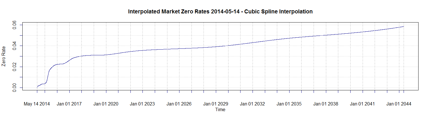
plot(x = termStruct.spline.interpolate[, “ZeroRate”], xlab = “Time”,
ylab = “Zero Rate”,
main = “Interpolated Market Zero Rates 2014-05-14 –
Cubic Spline Interpolation”,
ylim = c(0.0, 0.06), major.ticks= “years”,
minor.ticks = FALSE, col = “darkblue”)
This gives us a reasonably smooth curve, preserving the monotonicity of our data points:
c) Implement functions for discount factors and forward rates
We will now implement these functions, utilizing equations (A), (B), and (C) above. We will also take advantage of the functional programming feature in R, by incorporating the Actual / 365 Fixed day count as a functional argument, as an example. One could of course implement any other day count convention as a function of two lubridate dates, and pass it in as an argument.
First, let’s implement the Actual / 365 Fixed day count as a function:
# Simple example of a day count function: Actual / 365 Fixed
# date1 and date2 are assumed to be lubridate dates, so that we can
# easily carry out the subtraction of two dates.
dayCountFcn_Act365F <- function(date1, date2)
{
yearFraction <- as.numeric((date2 - date1)/365)
return(yearFraction)
}
Next, since the forward rate R(t, T) depends on the forward discount factor P(t, T), let’s implement the latter first:
# date1 and date2 are again assumed to be lubridate dates.
fwdDiscountFactor <- function(anchorDate, date1, date2, xtsMarketData, dayCountFunction)
{
# Convert lubridate dates to base R dates in order to use as xts indices.
xtsDate1 <- as.Date(date1)
xtsDate2 <- as.Date(date2)
if((xtsDate1 > xtsDate2) | xtsDate2 > max(index(xtsMarketData)) |
xtsDate1 < min(index(xtsMarketData)))
{
stop(“Error in date order or range”)
}
# 1st, get the corresponding market zero rates from our
# interpolated market rate curve:
rate1 <- as.numeric(xtsMarketData[xtsDate1]) # R(0, T1)
rate2 <- as.numeric(xtsMarketData[xtsDate2]) # R(0, T2)
# P(0, T) = exp(-R(0, T) * (T – 0)) (A), with t = 0 <=> anchorDate
discFactor1 <- exp(-rate1 * dayCountFunction(anchorDate, date1))
discFactor2 <- exp(-rate2 * dayCountFunction(anchorDate, date2))
# P(t, T) = P(0, T) / P(0, t) (C), with t <=> date1 and T <=> date2
fwdDF <- discFactor2/discFactor1
return(fwdDF)
}
Finally, we can then write a function to compute the forward interest rate:
# date1 and date2 are assumed to be lubridate dates here as well.
fwdInterestRate <- function(anchorDate, date1, date2, xtsMarketData, dayCountFunction)
{
if(date1 == date2) {
fwdRate = 0.0 # the trivial case
} else {
fwdDF <- fwdDiscountFactor(anchorDate, date1, date2,
xtsMarketData, dayCountFunction)
# R(t, T) = -log(P(t, T)) / (T – t) (B)
fwdRate <- -log(fwdDF)/dayCountFunction(date1, date2)
}
return(fwdRate)
}
d) Calculate discount factors and forward interest rates
As an example, suppose we want to get the five year forward three-month discount factor and interest rates:
# Five year forward 3-month discount factor and forward rate:
date1 <- anchorDate + years(5)
date2 <- date1 + months(3)
fwdDiscountFactor(anchorDate, date1, date2, termStruct.spline.interpolate,
dayCountFcn_Act365F)
fwdInterestRate(anchorDate, date1, date2, termStruct.spline.interpolate,
dayCountFcn_Act365F)
# Results are:
# [1] 0.9919104
# [1] 0.03222516
We can also check the trivial case for P(T, T) and R(T, T), where we get 1.0 and 0.0 respectively, as expected:
# Trivial case:
fwdDiscountFactor(anchorDate, date1, date1, termStruct.spline.interpolate,
dayCountFcn_Act365F) # returns 1.0
fwdInterestRate(anchorDate, date1, date1, termStruct.spline.interpolate,
dayCountFcn_Act365F) # returns 0.0
Finally, we can verify that we can recover the market rates at various points along the curve; here, we look at 1Y and 30Y, and can check that we get 0.0165 and 0.0585, respectively:
# Check that we recover market data points:
oneYear <- anchorDate + years(1)
thirtyYears <- anchorDate + years(30)
fwdInterestRate(anchorDate, anchorDate, oneYear,
termStruct.spline.interpolate,
dayCountFcn_Act365F) # returns 1.65%
fwdInterestRate(anchorDate, anchorDate, thirtyYears,
termStruct.spline.interpolate,
dayCountFcn_Act365F) # returns 5.85%
Concluding Remarks
We have shown how one can implement a term structure of interest rates utilizing tools available in the R packages lubridate and xts. We have, however, limited the example to interpolation within the 30 year range of given market data without discussing extrapolation in cases where forward rates are needed beyond the endpoint. This case does arise in risk management for longer term financial instruments such as variable annuity and life insurance products, for example. One simple-minded — but sometimes used — method is to fix the zero rate that is given at the endpoint for all dates beyond that point. A more sophisticated approach is to use the financial cubic spline method as described in the paper by Adams (2001), cited in part 1 of the current discussion. However, xts unfortunately does not provide this interpolation method for us out of the box. Writing our own implementation might make for an interesting topic for discussion down the road — something to keep in mind. For now, however, we have a working term structure implementation in R that we can use to demonstrate derivatives pricing and risk management models in upcoming articles.
R-bloggers.com offers daily e-mail updates about R news and tutorials about learning R and many other topics. Click here if you're looking to post or find an R/data-science job.
Want to share your content on R-bloggers? click here if you have a blog, or here if you don't.