I’ve been doing a lot of analyses recently that need rasters representing features in the landscape. In most cases, these data have been supplied as shapefiles, so I needed to quickly extract parts of a shapefile dataset and convert them to a raster in a standardised format. Preferably with as little repetitive coding as possible. So I created a simple and relatively flexible function to do the job for me.

The function requires two main input files: the shapefile (shp) that you want to convert and a raster that represents the background area (mask.raster), with your desired extent and resolution. The value of the background raster should be set to a constant value that will represent the absence of the data in the shapefile (I typically use zero).

The function steps through the following:

1. Optional: If shp is not in the same projection as the mask.raster, set the current projection (proj.from) and then transform the shapefile to the new projection (proj.to) using transform=TRUE.
2. Convert shp to a raster based on the specifications of mask.raster (i.e. same extent and resolution).
3. Set the value of the cells of the raster that represent the polygon to the desired value.
4. Merge the raster with mask.raster, so that the background values are equal to the value of mask.raster.
5. Export as a tiff file in the working directory with the label specified in the function call.
6. If desired, plot the new raster using map=TRUE.
7. Return as an object in the global R environment.

The function is relatively quick, although is somewhat dependant on how complicated your shapefile is. The more individual polygons that need to filtered through and extracted, the longer it will take.

shp2raster <- function(shp, mask.raster, label, value, transform = FALSE, proj.from = NA,
    proj.to = NA, map = TRUE) {
    require(raster, rgdal)

    # use transform==TRUE if the polygon is not in the same coordinate system as
    # the output raster, setting proj.from & proj.to to the appropriate
    # projections
    if (transform == TRUE) {
        proj4string(shp) <- proj.from
        shp <- spTransform(shp, proj.to)
    }

    # convert the shapefile to a raster based on a standardised background
    # raster
    r <- rasterize(shp, mask.raster)
    # set the cells associated with the shapfile to the specified value
    r[!is.na(r)] <- value
    # merge the new raster with the mask raster and export to the working
    # directory as a tif file
    r <- mask(merge(r, mask.raster), mask.raster, filename = label, format = "GTiff",
        overwrite = T)

    # plot map of new raster
    if (map == TRUE) {
        plot(r, main = label, axes = F, box = F)
    }

    names(r) <- label
    return(r)
}

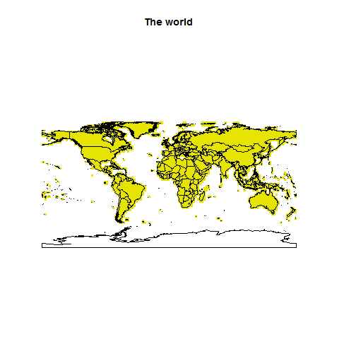
Below is a trivial example based on some readily available data in the maptools and biomod2 packages. Here I load a raster and a shapefile that represent our background of interest and foreground feature, respectively, and then plot them.

library(maptools)
library(raster)

## example: import world raster from package biomod2 and set the background
## values to zero
worldRaster <- raster(system.file("external/bioclim/current/bio3.grd", package = "biomod2"))
worldRaster[!is.na(worldRaster)] <- 0
plot(worldRaster, axes = F, box = F, legend = F, main = "The world")

# import world polygon shapefile from package maptools
data(wrld_simpl, package = "maptools")
plot(wrld_simpl, add = T)

One of the nice things about working with shapefiles in R is that you can subset the data based on attribute data the same way that you would any dataframe. This is really useful when combined with the shp2raster function as it means that we only need to convert the parts of the shapefile that we are actually interested in. For example, you may wish to create separate rasters for different landuse types that are contained in one shapefile as polygons with different attributes. You can see this in the trivial example below where I create two rasters from our world polygon data that select specific countries to convert based on the attribute NAME in the wrld_simpl shapefile.

# extract all Australian polygons and convert to a world raster where cells
# associated with Australia have a value of 1 and everything else has a
# value of 0.
australia <- shp2raster(shp = wrld_simpl[grepl(c("Australia";), wrld_simpl$NAME), ],
    mask.raster = worldRaster, label = "Where Amy currently lives", transform = FALSE, value = 1)

## Found 1 region(s) and 97 polygon(s)

# extract Australia, NZ & USA and convert to a world raster where cells
# associated with these countries have a value of 3 and everything
# else has a value of 0.
aus.nz.us <- shp2raster(shp = wrld_simpl[grepl(c("Australia|New Zealand|United States"),
    wrld_simpl$NAME), ], mask.raster = worldRaster, label = "All countries Amy has lived in",
    transform = FALSE, value = 3)

## Found 5 region(s) and 384 polygon(s)

Clearly these are quite trivial examples, where the raster and polygon layers don’t match very well (I mean, what is that blob of four pixels that represents my home country?!). But you hopefully get the general idea. In this case, I haven’t needed to do any transformation of the projections.

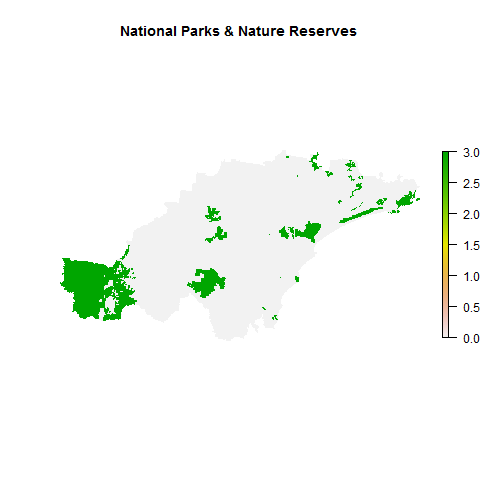
Below is an example where I was interested in creating a layer that represented protected areas within the Hunter Valley, Australia, for a conservation planning exercise. The available shapefile represented four different reserve types (National Parks, Nature Reserves, Regional parks and State Conservation Areas). In this case, the initial mask and polygon layers were in different projections, so I converted the shapefile to the correct projection by using transform=TRUE and proj.from and proj.to in the shp2raster call. I also wanted to extract a subset of the reserve types contained within the shapefile that related to National Parks (NP) and Nature Reserves (NR). The protected areas of interest needed to have a value of 3, while the background raster has a value of 0. Unfortunately I can’t supply the original layers but a real example of the code in action and the output map are below.

# set relevant projections
GDA94.56 <- CRS("+proj=utm +zone=56 +south +ellps=GRS80 +towgs84=0,0,0,0,0,0,0 +units=m +no_defs")
GDA94 <- CRS("+proj=longlat +ellps=WGS84 +datum=WGS84 +no_defs")

LH.mask <- raster("LH.mask.tif")
# set the background cells in the raster to 0
LH.mask[!is.na(LH.mask)] <- 0

NPWS.reserves <- readShapePoly("NPWSReserves.shp", proj4 = GDA94)

# convert the NPWS.reserves polygon data for National Parks & Nature
# Reserves to a raster, after changing the projection.
NPWS.raster <- shp2raster(shp = NPWS.reserves[grepl(c("NP|NR"), NPWS.reserves$reservetyp),],
    mask.raster = LH.mask, label = "National Parks & Nature Reserves", value = 3,
    transform = TRUE, proj.from = GDA94, proj.to = GDA94.56)

## Found 111 region(s) and 837 polygon(s)

The function should work with both polygon and polyline data. You can also use point data if you buffer it by a small amount first to create tiny polygons around the points. I’d pick a buffer size that makes sense relative to the resolution of the mask.raster.

Go forth and convert! Feedback on improvements definitely welcome – please leave a comment.