This post builds on my last: Alternatives to model diagnostics for statistical inference?, where I had claimed that we could make quality inferences about the best linear approximation to a quadratic relationship. The R code below implements such a scenario, to establish a framework for discussion. I have inserted comments to augment the code.

set.seed(42)
# Consider an infinite population where the association
# between two variables x and y is described by the following:
# y = x^2 + e 
# x ~ U(0, 15)
# e ~ N(0, 10)

# We seek a linear approximation of the relationship between
# x and y that takes the form below, and minimizes the average
# squared deviation (i.e., the 'best' approximation).
# hat(y) = a + b*x

# This function simulates "n" observations from the population.
simulate <- function(n=20) {
  x <- runif(n, 0, 15)
  y <- rnorm(n, x^2, 10)
  data.frame(y=y,x=x)
}

# This function finds the 'sample' best linear approximation to the
# relationship between x and y.
sam_fit <- function(dat)
  lm(y ~ x, data=dat)

# We can approximate the 'population' best linear approximation by
# taking a very large sample. Note that this only works well for 
# statistics that converge to a population quantity.
pop_fit <- sam_fit(simulate(1e6))

## > pop_fit
## 
## Call:
## lm(formula = y ~ x, data = simulate(1e+06))
## 
## Coefficients:
##   (Intercept)            x  
##        -37.53        15.00  

The figure below illustrates the true quadratic curve and the best linear approximation (pop_fit), overlaid against 10000 samples.

# This function creates a level confidence region for the intercept
# and slope of the best linear approximation, and tests whether
# the region includes the corresponding population values.
# The 'adj' parameter adjusts the critical value, making the 
# confidence region larger or smaller.
sam_int <- function(dat, val=c(a=0, b=0), level=0.95, adj=0.00) {
  s <- sam_fit(dat)
  d <- coef(s) - val
  v <- vcov(s)
  c <- qchisq(level+adj, 2)
  as.numeric(d %*% solve(v) %*% d) < c
}

# By specifying that the region has 95% confidence, we intend that
# the region includes the population quantity in 95% of samples.
# We can assess the coverage of the above 95% confidence region by
# drawing repeated samples from the population and checking whether
# the associated confidence regions include the population values:
coverage20 <- mean(replicate(1e4, sam_int(simulate(20),
                                             val=coef(pop_fit))))

## > coverage20
## [1] 0.855

# Because the true coverage is less than the nominal coverage,
# the confidence region is anti-conservative. However, suppose that
# we can adjust the critical value of the region so that the true
# coverage is equal to the nominal value:
coverage20a <- mean(replicate(1e4, sam_int(simulate(20),
                                              val=coef(pop_fit),
                                              adj=0.045)))

## > coverage20a
## [1] 0.9476

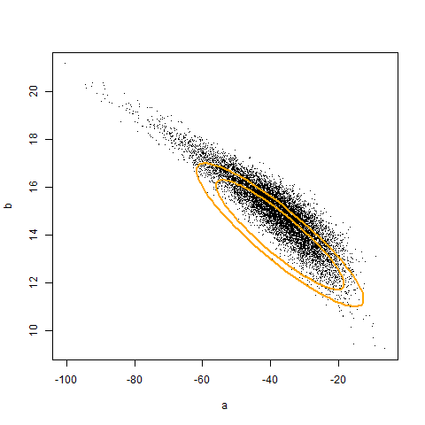
The code above illustrates that if we had access to a population, we can adjust the coverage of a confidence region to be correct. The animation (created using Yihui’s animation package) below illustrates the original and corrected confidence regions for ten different samples of size 20, overlaid against 10000 sample estimates of a and b. Unfortunately, we don’t generally have access to the population. Hence, the adjustment must be made by an alternative, empirical, mechanism. In the next post, I will show how to use iterated Monte Carlo (specifically the double bootstrap) to make such an adjustment.